Overview
CalEyeZ removes the friction from nutrition tracking. The user places food on a scale and takes one photo; the system returns calories and a macronutrient breakdown automatically. It solves two independent engineering problems and proves each one with data.
The two questions
| Question | Engineering problem | Solution (proven) |
|---|---|---|
| What is it? | Identify the food, including local Israeli dishes that international models never saw, without the catastrophic forgetting that ruined a single combined model. | A Global expert (132 classes) and an Israeli expert (13 classes), combined by a learned XGBoost arbiter. See Arbiter. |
| How much? | Obtain an accurate mass from a single photo. | Read the mass directly from a reverse-engineered BLE scale, after five vision based volume methods were measured and rejected. See Validation. |
Pitch, audience, goals
- Pitch: point a camera at a plate, get its nutrition. No manual logging, no barcode, no portion guessing.
- Target audience: people managing intake for health reasons (diabetes, fitness, clinical diet) who abandon manual calorie apps because logging is tedious and portion estimates are wrong.
- Primary goal: end-to-end food recognition above the 80% FRS requirement, on a strictly held-out, leakage-free test set. Met at 86.2% (V2 system) and 88.18% (Global model alone).
- Secondary goal: accurate weight without asking the user to type anything. Met by BLE.
Run-time architecture
Edge desktop application in Python with a CustomTkinter GUI. Inference runs locally on an NVIDIA GPU; only the nutrient lookup uses the network.
Key project risks (tracked)
| Risk | Why it matters | Status |
|---|---|---|
| Catastrophic forgetting when adding local food | One combined model lost accuracy on both old and new classes | controlled by the two-expert split |
| Data leakage inflating accuracy | Duplicate images across splits make the test score a lie | removed by exact + perceptual de-dup |
| Class imbalance hurting rare classes | Ingredient classes have far fewer images than dishes | measured and reported per class |
| Arbiter sending the image to the wrong expert | A wrong decision wastes a correct prediction | 4.91% of images, fully decomposed |
| Weight error from vision volume estimation | Volume to mass fails on density | avoided by direct BLE reading |
The full risk-to-test mapping is in the Validation & Risks tab.
Then vs Now presented in class current
This tab compares exactly what was shown at the review conference against the
rebuilt system. Every "then" number is recomputed from the original results file
FINAL_REPORT_v3_results.csv (16,720 images); every "now" number is from the
current leakage-free evaluation.
Headline comparison
| Metric | Then (class) | Now | Change | Note |
|---|---|---|---|---|
| Full system top-1 | 80.30% | 86.2% (V2) | +5.9 | clean data + V2 open-set arbiter |
| Global model top-1 (own domain) | 84.6% | 88.18% | +3.58 | apples to apples: each model on its own classes (158 then, 132 now). 84.6% is the as-presented figure; recomputed on this CSV it is 82.2% |
| Always-global baseline (full mix) | 76.43% | 77.98% | +1.55 | using only the global model on every image, including Israeli food it scores 0% on |
| Oracle ceiling (best possible arbiter) | 82.97% | 88.40% | +5.43 | headroom the models allow |
| Classes (global) | 158 to 161 | 132 | cleaned | merged, renamed, de-duplicated |
| Israeli expert classes | 8 | 13 (+background) | +5 | broader local coverage; V2 adds an open-set background class |
| Arbiter accuracy / ROC-AUC | 78.7% | 96.1% / 0.973 | better | the arbiter (XGBoost); V2 added i_p_background and lifted AUC 0.933 to 0.973 |
| Val vs test gap (leakage signal) | about 4 pts | 0.02 pt | closed | 88.16 val vs 88.18 test |
Why the old router barely used the second expert
In the class version the router chose the old model on 95.0% of images (15,877 of 16,720) and the new model only 5.0% of the time. The new expert was contributing only 6.54% correct answers, so the router had almost nothing to gain by switching. In other words it was not really routing, it was defaulting to the larger model. The current arbiter is a genuine decision maker, explained in full in the Arbiter tab.
| Router decision (then) | Count | Share |
|---|---|---|
| Chose OLD model | 15,877 | 95.0% |
| Chose NEW model | 843 | 5.0% |
The current arbiter is trained as an explicit domain detector
(route_to_israeli = (domain == israeli)), reaches Israeli recall of 79% with global
recall 98% in V2 (up from 61% / 98% after the open-set background retrain), and the
Arbiter tab explains exactly which features drive
each decision. It is also why the current component is correctly called an arbiter, not a
router: it adjudicates between two experts that have already run, rather than forwarding by a rule.
What changed structurally
| Area | Then | Now |
|---|---|---|
| Backbone | YOLOv8-cls, imgsz 224 | YOLO11l-cls, imgsz 320 |
| Calibration | asymmetric temperature scaling (T=0.55 / 1.0) to hide probability dilution | not needed; arbiter learns relative confidence directly |
| Data hygiene | no de-dup, leakage between splits | SHA-1 exact + 64-bit dHash perceptual de-dup, verified zero cross-split leaks |
| Reported metric | raw router accuracy | ROC-AUC + per-domain recall + full error decomposition |
Source files: FINAL_REPORT_v3_results.csv (then),
datasets/system_evaluation.csv and arbiter_dataset.csv (now).
Dataset
The global dataset was consolidated from the inconsistent 158-class set into a clean,
leakage-free 132-class label space, then re-split 70/20/10. This is where two of the reviewer's
points are answered directly: class balance and leakage. Pipeline:
scripts/flatten_general_dataset.py.
Where the classes went (158 to 132, fully accounted)
The reduction is not deletion of useful classes. Most removed labels either moved to the Israeli expert or were folded into a class they were visually identical to. Here is every change.
| Operation | Count | Detail | Reason |
|---|---|---|---|
| Moved to Israeli expert | 8 | baklava · bourekas_cheese · falafel · hummus · samosa · schnitzel · shakshuka · shawarma. Pita and plural variants (falafel_pita, shawarma_pita, samosas, bourekas) were merged into the base dish; two very rare dishes (hraime, knafeh) were dropped for too few images. | Local dishes left the global model and became the Israeli expert's job. They are not lost, they are handled by the other model and recovered by the arbiter |
| Merge | 8 | filet_mignon + prime_rib → steak · beef_tartare + tuna_tartare → tartare · frozen_yogurt → ice_cream · dumplings → gyoza · sweetcorn → corn · capsicum → bell_pepper | Classes humans cannot reliably separate in a photo only add confusion and split training data |
| Delete | 8 | baby_back_ribs · pork_chop · pulled_pork_sandwich (pork, out of scope) · paprika (mixed/noisy) · soy_beans (redundant with edamame) · beignets · huevos_rancheros · sweetpotato | Out of scope or unusable; noisy labels lower every other class's accuracy |
| Rename | 5 | potato → baked_potato · chilli_pepper → chili_pepper · jalepeno → jalapeno · raddish → radish · edame → edamame | Casing and spelling collisions created duplicate label folders (still present, just renamed) |
What each model is trained to recognize
The two experts cover disjoint label spaces. The global model knows 132 international foods; the Israeli model knows 13 local dishes. No class appears in both, which is why routing reduces cleanly to a domain decision.
Global model
- almonds
- apple
- apple pie
- avocado
- baked potato
- banana
- beef carpaccio
- beet salad
- beetroot
- bell pepper
- bibimbap
- brazil nuts
- bread pudding
- breakfast burrito
- bruschetta
- cabbage
- caesar salad
- canned tuna
- cannoli
- caprese salad
- carrot
- carrot cake
- cashews
- cauliflower
- ceviche
- cheese plate
- cheesecake
- chicken curry
- chicken quesadilla
- chicken wings
- chili pepper
- chocolate cake
- chocolate mousse
- churros
- clam chowder
- club sandwich
- coconut
- corn
- couscous
- crab cakes
- creme brulee
- croque madame
- cucumber
- cup cakes
- deviled eggs
- donuts
- edamame
- eggplant
- eggs benedict
- escargots
- fish and chips
- foie gras
- french fries
- french onion soup
- french toast
- fried calamari
- fried rice
- garlic
- garlic bread
- ginger
- gnocchi
- grapes
- greek salad
- grilled cheese sandwich
- grilled salmon
- guacamole
- gyoza
- hamburger
- hazelnuts
- hot and sour soup
- hot dog
- ice cream
- jalapeno
- kiwi
- lasagna
- lemon
- lettuce
- lobster bisque
- lobster roll sandwich
- macadamia
- macaroni and cheese
- macarons
- mango
- miso soup
- mussels
- nachos
- omelette
- onion
- onion rings
- orange
- oysters
- pad thai
- paella
- pancakes
- panna cotta
- pear
- peas
- pecans
- peking duck
- pho
- pine nuts
- pineapple
- pistachios
- pizza
- pomegranate
- poutine
- radish
- ramen
- ravioli
- red velvet cake
- risotto
- sashimi
- scallops
- seaweed salad
- shrimp and grits
- spaghetti bolognese
- spaghetti carbonara
- spinach
- spring rolls
- steak
- strawberry shortcake
- sushi
- tacos
- takoyaki
- tartare
- tiramisu
- tomato
- turnip
- waffles
- walnuts
- watermelon
- white rice
Israeli model
- baklava
- bourekas cheese
- falafel
- hummus
- jachnun
- malawach
- meorav yerushalmi
- sabich
- samosa
- schnitzel
- shakshuka
- shawarma
- sufganiyah
De-duplication: how leakage was removed
Two stages run before splitting, so the split unit is a content cluster and never a raw file:
- Exact: SHA-1 hash of file bytes. Byte-identical copies are dropped (981 found).
- Near-duplicate: 64-bit dHash with Hamming distance ≤ 5. Visual twins are clustered and the whole cluster is kept inside a single split.
| Split | Images | Share | Classes |
|---|---|---|---|
| train | 69,491 | 70.0% | 132 |
| val | 19,827 | 20.0% | 132 |
| test | 9,960 | 10.0% | 132 |
| total | 99,307 | 100% | 132 |
Class balance (the reviewer's point)
The classes are not perfectly balanced, and that is reported honestly rather than hidden. Dish classes hold roughly 750 to 1,000 images each; ingredient classes (single fruits, nuts) hold far fewer. The effect is confined to the smallest classes and is a small-sample effect, not a systematic weakness. The training uses class-aware sampling and heavy augmentation to compensate, and per-class recall is reported in the System Analysis tab so the imbalance is visible, not papered over.
Global Model 88.18% clean test
YOLO11l-cls (Ultralytics, ImageNet-1k pretrained, about 13M parameters),
fine-tuned on the 132-class set. Run directory: runs/general_model_flattened/.
Why this model, backed by data
| Decision | Alternatives | Why this one |
|---|---|---|
| YOLO11l-cls backbone | YOLOv8-cls (previous), ResNet-50, EfficientNet | Newer C3k2 backbone gave a higher clean top-1 at the same VRAM budget; classification head is simple to fine-tune and export |
| imgsz 320 (was 224) | 224, 416, 640 | 320 lifted top-1 over 224 while still fitting batch 16 in about 2.2 GB; 640 gave no measurable gain for far more compute |
| Heavy augmentation | light / default aug | Deliberate trade: a moderate-aug retrain scores about 90% on this clean test but is more brittle in the classroom. Robustness was chosen on purpose |
| Two experts, not one | single 145-class model | The single combined model lost accuracy on both old and new classes (catastrophic forgetting). Two experts plus an arbiter avoid it |
Training configuration and why we chose each setting
| Setting | Value | Why this choice |
|---|---|---|
| imgsz | 320 | Food is a fine-texture problem (rice grains, crumbs, sauce sheen). 320 beat the default 224 on top-1 while still fitting batch 16 on an 8 GB GPU; 640 gave no measurable gain for far more compute. |
| batch | 16 | The largest batch that fits comfortably at 320 px with AMP headroom, large enough for stable batch-norm and gradient estimates without gradient accumulation. |
| optimizer | AdamW + cosine LR | AdamW decouples weight decay from the adaptive step, which fine-tunes a pretrained backbone reliably; cosine annealing lowers the LR smoothly to a good minimum with no hand-tuned step schedule. |
| lr0 / lrf | 1e-3 / 0.01 | 1e-3 is the standard AdamW base for fine-tuning an ImageNet-pretrained backbone; lrf 0.01 decays to 1% of that by the end so late epochs refine the weights instead of thrashing them. |
| epochs / patience | 150, patience 30 (stopped 116) | A generous cap so the model is never under-trained, with early stopping so it does not waste compute; patience 30 tolerates the noisy validation plateau before stopping. |
| dropout | 0.2 | Regularises against overfitting the large dish classes (about 1,000 images each) given the heavy class imbalance. |
| label smoothing | 0.1 | Stops the model becoming over-certain on visually ambiguous pairs (mousse vs cake), which improves probability calibration. Better-calibrated confidences directly feed the arbiter's features. |
| AMP (mixed precision) | on (~2.2 GB) | Halves memory and speeds training with no accuracy loss, leaving VRAM headroom on the 8 GB card for the 320 px / batch 16 setup. |
| best epoch | 73 | best.pt is frozen at the validation peak, so the mild overfit that begins after about epoch 60 (train loss down, val loss up) never affects the reported number. |
Robustness to lighting and blur: the trade-off we chose on purpose
A model that scores well in a studio but fails on a darker plate is useless as a product. We therefore treated harsh, variable lighting as a first-class requirement and trained for it directly with aggressive photometric augmentation. On every training batch each image is re-lit at random, so the network never sees the "one true lighting" of a dish and is forced to learn features that are invariant to it.
| Augmentation | Value | What real-world condition it defeats |
|---|---|---|
hsv_v (brightness) | 0.50 | Exposure / dim vs bright light. Each image is shown with brightness ×U(0.5, 1.5) - from 50% darker to 50% brighter. This is the "darker plate" case, seen thousands of times. |
hsv_h (hue) | 0.02 | Colour temperature - warm tungsten vs cool fluorescent/daylight white balance. |
hsv_s (saturation) | 0.75 | Washed-out vs vivid colour under different lights (×U(0.25, 1.75)). |
| custom blur | p=0.35 | Motion/defocus/Gaussian blur (Albumentations) on 35% of batches: a live webcam is rarely perfectly sharp. 65% stay sharp so clean food is still learned. |
erasing | 0.40 | Random occlusion - glare spots, a hand, or clutter over part of the dish. |
degrees / scale / translate / flips | 20 / 0.60 / 0.15 / 0.5 | Pose invariance: food has no canonical orientation and the demo camera is hand-held and angled. |
How it works. Per image, Ultralytics samples a random gain and rescales the colour channels:
V ← V·U(0.5,1.5), S ← S·U(0.25,1.75),
H ← (H·U(0.98,1.02)) mod 180. Over the ~116 training epochs each photo is seen
~116 times, each time under a different random lighting, white balance and exposure.
Training code
# scripts/training/train_general_model.py  (essentials)
from ultralytics import YOLO

model = YOLO("yolo11l-cls.pt")            # ImageNet-1k pretrained
model.train(
    data="datasets/general_model_flattened",  # 132 classes, 70/20/10
    imgsz=320, batch=16, epochs=150, patience=30,
    optimizer="AdamW", lr0=1e-3, lrf=0.01, cos_lr=True,
    dropout=0.2, label_smoothing=0.1,
    augment=True, hsv_h=0.02, hsv_s=0.75, hsv_v=0.50,  # lighting/temp/exposure
    degrees=20, translate=0.15, scale=0.60, flipud=0.15, fliplr=0.50, erasing=0.40,
    # + custom Albumentations blur (motion/defocus/gaussian) on 35% of batches via a train-batch callback
    project="runs", name="general_model_flattened",
)
# validate on the held-out TEST split
model.val(data="datasets/general_model_flattened", split="test")
Results (best.pt, epoch 73)
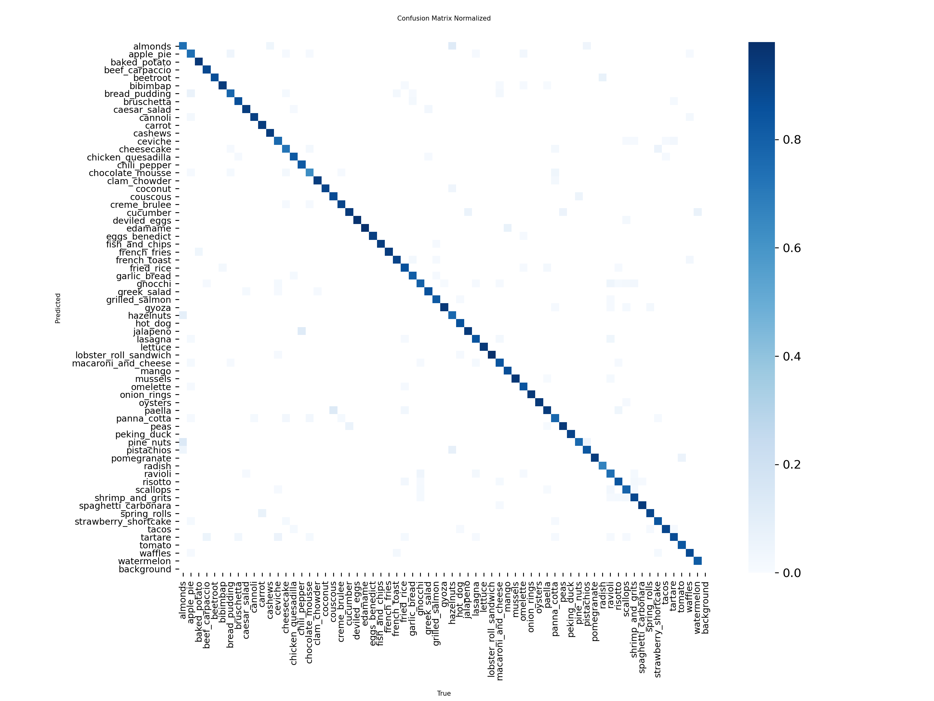
Most-confused class pairs (test)
Every meaningful confusion is a plausible visual overlap, not a failure:
| True → Predicted | Rate |
|---|---|
| chocolate_mousse → chocolate_cake | 12% |
| apple_pie → bread_pudding | 10% |
| gnocchi ↔ ravioli | 7% |
| beef_carpaccio → tartare | 6% |
| lobster_bisque ↔ clam_chowder | 5% |
Israeli Model 91.7% on its domain
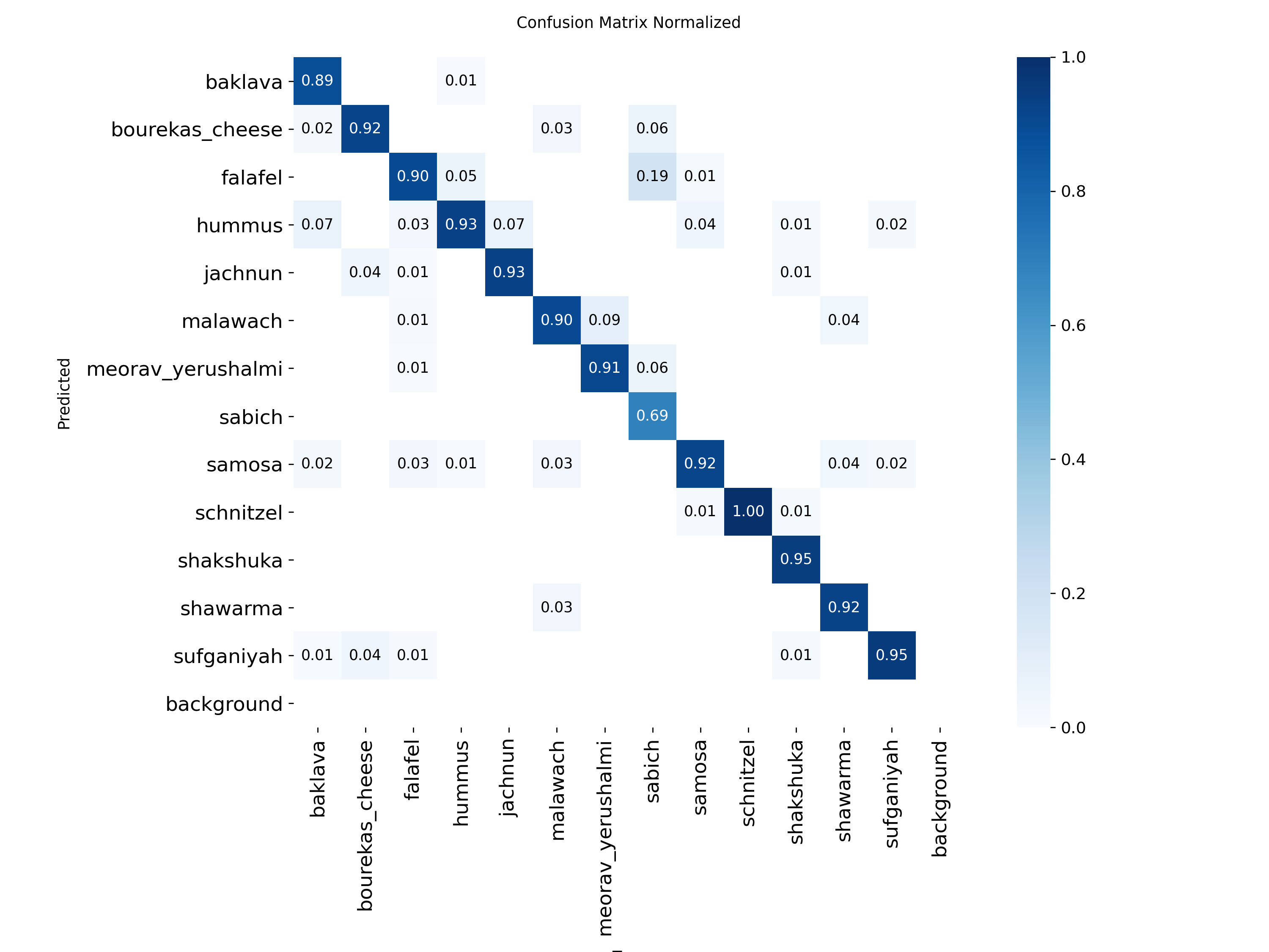
YOLO11l-cls, 13 Israeli classes (baklava, bourekas_cheese, falafel, hummus,
jachnun, malawach, meorav_yerushalmi, sabich, samosa, schnitzel, shakshuka, shawarma, sufganiyah).
Run: runs/israeli_food_yolo11l/, imgsz 224.
Why a second, separate expert
The first attempt added Israeli food to the global model and retrained. The combined model got confused: it lost accuracy on both the international classes it already knew and the new local ones. This is catastrophic forgetting, and it was the trigger for the whole arbiter architecture. Keeping the Israeli dishes in their own small expert means the global model never degrades, and the local model can specialise hard on a narrow domain where it reaches about 92% while the global model scores 0% on those same classes.
Training configuration and why we chose each setting
| Setting | Value | Why this choice |
|---|---|---|
| backbone | YOLO11l-cls | The same backbone as the global model so both experts produce comparable confidence and embedding features, which keeps the arbiter's inputs consistent across the two models. |
| classes | 13 | A narrow, curated local-cuisine set. Keeping the domain small lets this expert specialise hard and reach about 92% where the global model scores 0% on the same dishes. |
| imgsz | 224 | Lower than the global model's 320 because the dataset is much smaller; 224 trains fast, avoids overfitting the limited data, and the local dishes are distinguishable at this resolution. |
| epochs | 63 (best 59) | The small dataset converges quickly, so a short schedule is enough; best.pt is frozen at epoch 59 (the validation peak) before the noisy tail. |
| data | datasets/israeli-food-master | A dedicated, hand-collected local-food set, kept separate from the global data so adding local cuisine never degrades the global model (no catastrophic forgetting). |
| best top-1 | 91.70% | Strong on its own domain (top-5 about 99%), which is what makes the two-expert split worthwhile. Its out-of-domain overconfidence is handled by the arbiter, not by this model. |
Results
The accuracy curve is noisier than the global model's because the dataset is much smaller, so each epoch sees fewer images and the validation estimate has higher variance. The trend is still a clean climb to about 92%.
Known behaviour the arbiter must handle
Arbiter acc 96.1%, ROC-AUC 0.97 (V2)
Why we call it an arbiter, not a router
A router would forward the image to one model based on a fixed rule before seeing any result. Our component does the opposite: it runs both experts first, then weighs their competing evidence (confidence, entropy, margin) and adjudicates which one to trust. That is arbitration, not routing. The distinction matters because the decision is made on the models' actual behaviour for this specific image, not on a prior guess about where the image should go.
What the arbiter is, in one paragraph
The arbiter is not a third food classifier. It never looks at the image. It looks only at
the two experts' output behaviour for that image (their confidences, how spread out their guesses
are, how decisive each one is) and answers a single yes/no question: does this image belong to
the Israeli expert's domain? If yes, the system returns the Israeli model's label; if no, it
returns the global model's label. Formally the target is
route_to_israeli = (domain == israeli). Because the two label spaces do not overlap,
routing reduces cleanly to domain detection.
The 20 features and their math
The arbiter input is a 20-number vector: 7 numbers summarising the Global model's output, 8 for the
Israeli model (V2 adds i_p_background), and 5 interaction terms that compare the two. Below,
p_k is the k-th highest softmax probability and K the number of classes. The
"g_" prefix is the Global model, "i_" the Israeli model.
| # | Feature | Meaning | Formula |
|---|---|---|---|
| 1-5 | g_conf1 … g_conf5 | Global model's top-5 class probabilities | top-5 of softmax(global) |
| 6 | g_entropy | How spread out the Global guess is (low = decisive) | −Σ p_i · ln(p_i) |
| 7 | g_margin | How decisive the Global top guess is | g_conf1 − g_conf2 |
| 8-12 | i_conf1 … i_conf5 | Israeli model's top-5 class probabilities | top-5 of softmax(israeli) |
| 13 | i_entropy | Spread of the Israeli guess | −Σ p_i · ln(p_i) |
| 14 | i_margin | Decisiveness of the Israeli top guess | i_conf1 − i_conf2 |
| 15 | i_p_background (V2) | Israeli model's "not one of my dishes" probability. High = route to global. Now the #1 feature by gain (0.289). | softmax(israeli)[background] |
| 16 | conf_gap | Which expert is more confident at the top | g_conf1 − i_conf1 |
| 17 | conf_ratio | Relative top-1 confidence (scale-free) | g_conf1 / (i_conf1 + 1e-6) |
| 18 | entropy_gap | Who is more uncertain (>0 = Israeli more uncertain) | i_entropy − g_entropy |
| 19 | margin_gap | Whose decision is sharper | g_margin − i_margin |
| 20 | both_unsure | Flag: neither expert is confident | 1 if (g_conf1<0.5 and i_conf1<0.5) else 0 |
i_p_background (gain 0.289), then the interaction
terms. They encode relative behaviour, which is what actually separates the domains.
i_p_background, entropy_gap and conf_gap rank highest by
importance: the arbiter trusts the Israeli model when it is confident, the Global model is comparatively
uncertain, and the Israeli model is not signalling "background". That open-set signal is exactly
why V2 survives the Israeli model's out-of-domain overconfidence and lifted routing AUC from 0.933 to
0.973.Seeing the math live (per image)
The demo does not just print a probability. For each capture it computes the exact TreeSHAP contribution of every feature, that is, how many log-odds each one added toward "route to Israeli", and shows the top contributors under the decision panel. A typical readout for a global food:
WHY (top feature contributions):
conf_gap     =  0.640  +1.31 -> Global    # global far more confident than israeli
entropy_gap  = -0.220  +0.74 -> Global    # israeli more uncertain than global
i_conf1      =  0.180  +0.42 -> Global    # israeli top-1 is weak
This is the faithful per-prediction explanation (not a global average), so during the demo you can point at the exact numbers that produced the routing decision.
The arbiter decides on relative confidence between the experts, not on the Israeli model's raw confidence, which is exactly why it survives that model's out-of-domain overconfidence.
The softmax behind the features (with code proof)
Every confidence the arbiter consumes is a softmax probability. Softmax turns a model's raw
logits z into a probability distribution over classes:
softmax(z)_i = e^(z_i) / Σ_j e^(z_j) # non-negative, sums to 1
Where it runs: we do not hand-write softmax. Each YOLO11l-cls expert applies it inside its
classification head (Ultralytics / PyTorch), so results.probs is already a softmax
distribution. Our pipeline consumes that output and derives the features from it. Proof, straight
from scripts/arbiter/generate_arbiter_dataset.py (identical in the live demo's
expert_features):
probs     = r.probs                          # the Classify head's softmax output
top5_conf = [float(c) for c in probs.top5conf.tolist()]   # top-5 softmax probabilities
full      = probs.data.cpu().numpy()         # the full softmax vector (sums to 1)
full      = np.clip(full, 1e-12, 1.0)        # guard log(0)
entropy   = float(-(full * np.log(full)).sum())           # H = -Σ p ln p
margin    = float(top5_conf[0] - top5_conf[1])        # p1 - p2
So g_conf1..5 / i_conf1..5 are softmax probabilities, *_entropy
is the entropy of the softmax vector, *_margin is the gap between its top two, and
i_p_background is the softmax mass on the background class. All 20 features are functions
of these two softmax distributions, never the raw logits.
P(israeli) = 1 / (1 + e^(-logit)). The live demo recovers
that logit with logit = ln(p / (1 - p)) to show the math panel. In short: the experts
use softmax (proof above); the arbiter uses its sigmoid sibling.Why XGBoost, backed by data
A Random Forest looked great on training data but collapsed on held-out data: it memorised. XGBoost gave essentially the same test accuracy with a tiny generalisation gap, so it was chosen.
| Metric | Random Forest | XGBoost (chosen) | Conclusion |
|---|---|---|---|
| Train accuracy | 98.1% | 81.2% | RF overfit badly; XGBoost is stable, so it was selected |
| Test accuracy | 78.6% | 78.7% | |
| Overfit gap | 19.5% | 2.5% |
Those figures are from the earlier router study; the current V2 arbiter keeps XGBoost and reaches routing accuracy 96.07% and ROC-AUC 0.973 on the rebuilt dataset (with the i_p_background feature).
Training code
# scripts/arbiter/train_arbiter_xgb.py  (essentials)
import xgboost as xgb, pandas as pd

df = pd.read_csv("datasets/arbiter_dataset.csv")   # both models over val+test
y  = (df.domain == "israeli").astype(int)        # route_to_israeli target

# features: each model's conf/entropy/margin + interaction deltas
X = df[["g_conf1","g_entropy","g_margin",
        "i_conf1","i_entropy","i_margin",
        "conf_gap","conf_ratio","entropy_gap","margin_gap"]]

train = df.split == "val"                          # train on val rows
test  = df.split == "test"                         # evaluate on test rows

clf = xgb.XGBClassifier(
    n_estimators=400, max_depth=4, learning_rate=0.05,
    subsample=0.8, colsample_bytree=0.8,
    scale_pos_weight=0.5,                         # Israeli minority ~7%
    eval_metric="auc", early_stopping_rounds=30)
clf.fit(X[train], y[train], eval_set=[(X[test], y[test])])
clf.save_model("scripts/arbiter/arbiter_xgb.json")
Results (V2 arbiter)
P(israeli) for every image. We sweep a decision threshold from high to low; at each setting
we plot two numbers: how many Israeli images it correctly catches (the True Positive Rate,
up) against how many global images it wrongly sends to the Israeli model (the False Positive
Rate, right). Joining those points draws the ROC curve. The area under that curve (AUC)
is a single 0-1 score: 1.0 = perfect separation, 0.5 = a coin flip (the dashed
diagonal). Equivalently, AUC is the probability the arbiter ranks a random Israeli image above a random
global one. A curve that hugs the top-left corner is better - it catches Israeli images
without misrouting global ones.How to read it. This is the real V2 routing ROC,
computed on the 11,352-image held-out test set (route_prob_israeli vs. true
domain in datasets/system_evaluation.csv). The teal curve shoots almost straight up the
left edge then runs along the top - it catches most Israeli images while misrouting very few
global ones. The area beneath it is 0.973.
Why it matters here. Moving the threshold just slides you along one
curve (more Israeli caught costs more global misrouted - zero-sum). The only way to win net
accuracy is to lift the whole curve, i.e. raise the AUC. V2's open-set
i_p_background signal did exactly that: 0.933 → 0.973.
ROC-AUC in one line: the probability that the arbiter gives a randomly chosen Israeli image a higher P(israeli) than a randomly chosen global image. 1.0 is perfect separation, 0.5 is a coin flip. 0.973 means it ranks the two domains correctly 97% of the time. Recall = the share of each domain it actually catches.
| Routing metric (test) | V1 | V2 |
|---|---|---|
| Routing accuracy | 93.40% | 96.07% |
| ROC-AUC | 0.933 | 0.973 |
| Israeli recall | 61.3% | 79.2% |
| Global recall | 97.6% | 98.4% |
| System top-1 (test) | V1 | V2 |
|---|---|---|
| Always-global baseline | 78.0% | 77.4% |
| Arbiter (routed) | 83.8% | 86.2% |
| Oracle ceiling | 88.7% | 88.8% |
| Arbiter gain | +5.8 | +8.8 pts |
- The problem in V1: the Israeli model was overconfident on non-Israeli food (it would call a bowl of risotto "hummus" at 80%+). So its confidence was a noisy, untrustworthy signal, the arbiter learned to discount it and default to the global prior, and Israeli recall stalled at 61%.
- The fix (open-set retrain): we retrained the Israeli model with a 14th
backgroundclass of non-Israeli food, so it now answers "this is not one of my dishes" instead of forcing a guess. Measured: its meanP(background)is 0.50 on global food vs 0.03 on real Israeli food, a near-clean separator. - Exposed to the arbiter as one feature:
i_p_background. It instantly became the arbiter's #1 feature by gain (0.289), ahead of every confidence/entropy term. - Why this is a real win, not a knob turn: earlier analysis showed that simply moving the decision threshold is near zero-sum (every Israeli image won costs a global image). The only way to gain net accuracy is to raise the ROC-AUC, which needs new information. The background signal did exactly that: AUC 0.933 to 0.973, Israeli recall 61% to 79%, system 83.8% to 86.2%, with global recall holding. The earlier note that "better model calibration would raise Israeli recall, more arbiter tuning would not" is precisely what V2 confirmed.
scripts/arbiter/arbiter_xgb.json (V2, 20 features). See the Israeli Model V2 tab
for the full retrain and the per-class numbers.CNN Visualizer: what the layers do to one image
This is a live, step-by-step view of how a convolutional classifier turns pixels into a class. Pick an input, then press Play. The same logic runs inside the YOLO11 backbone, just with many more filters and layers.
The exact layers in our model - YOLO11l-cls, start to end
This is not a generic diagram: the table is read directly from our trained
best.pt by pushing one 320×320×3 image through the network and recording the
output tensor of every block. Our Global model is 11 top-level blocks (which expand to
309 individual layers such as Conv/BatchNorm/SiLU/Linear) and 13.0 million parameters.
Resolution shrinks 320→10 while channel depth grows 3→512: the network trades spatial detail
for semantic depth, then the head turns the final 512-vector into 132 class probabilities.
| # | Block | Output (C×H×W) | Params | What it does |
|---|---|---|---|---|
| 0 | Conv (stem) | 64 × 160 × 160 | 1,856 | First convolution, stride 2 halves the image; learns 64 low-level filters (edges, colour blobs) - exactly the kernels in the panels below. |
| 1 | Conv | 128 × 80 × 80 | 73,984 | Downsample again and widen to 128 channels (more filter types). |
| 2 | C3k2 | 256 × 80 × 80 | 173,824 | CSP block: splits the features, runs a stack of small bottleneck convs, concatenates. Builds textures from edges. |
| 3 | Conv | 256 × 40 × 40 | 590,336 | Downsample to 40×40. |
| 4 | C3k2 | 512 × 40 × 40 | 691,712 | Deeper features → small object parts; widen to 512 channels. |
| 5 | Conv | 512 × 20 × 20 | 2,360,320 | Downsample to 20×20. |
| 6 | C3k2 | 512 × 20 × 20 | 2,234,368 | Mid-level semantic features (combinations of parts). |
| 7 | Conv | 512 × 10 × 10 | 2,360,320 | Final downsample to a 10×10 grid. |
| 8 | C3k2 | 512 × 10 × 10 | 2,234,368 | High-level features (whole-object concepts). |
| 9 | C2PSA | 512 × 10 × 10 | 1,455,616 | YOLO11's attention block (position-sensitive self-attention): lets distant regions of the plate inform each other before the decision. |
| 10 | Classify (head) | 132 | 827,012 | Global-average-pool the 512 maps into one 512-vector → dropout → Linear(512→132) → softmax = class probabilities. This is the fingerprint + weights stages below. |
The Israeli expert is the identical YOLO11l-cls backbone but fed 224×224 (so the grid is 112→7 instead of 160→10) with a 14-class head - 11 blocks, 12.85M parameters. The four stages below zoom into what happens inside these blocks, and the last stage runs the block-0 style filters on a real photo you upload.
Layer 1 · Convolution (feature extraction)
A small grid of weights (the kernel) slides across the image. At each position it multiplies the overlapping pixels by the weights and sums them. That single number becomes one pixel of the output feature map. Different kernels detect different things: edges, colours, textures.
Layers 2 to N · Stacking and pooling (from edges to concepts)
Early layers find edges and colour blobs. Stacking convolutions and downsampling (pooling) lets later layers combine those into textures, then parts, then whole concepts like "rice grains" or "round red object". Each box below is a feature map at increasing depth and decreasing resolution.
Bottleneck · The latent vector (the image's signature)
After the last conv block the whole image is compressed into one long vector of numbers (1280 in this backbone). Lit cells are features that are strongly active for this image. This vector is the image's fingerprint; two photos of the same dish produce similar vectors.
Classifier · Weights turn the signature into a decision
The final layer holds one weight template per class. It takes the dot product of the latent vector with each class template; the class whose template matches best wins. Softmax then turns the scores into probabilities. These templates are literally "the weights".
On a real photo · run the filters and see the outcome after each one
Everything above used a tiny synthetic image so the arithmetic was visible. Here it runs for real: upload any food photo and the browser applies real 3×3 convolution kernels to it - exactly the operation the first layer of the YOLO11 backbone performs. Each panel below is the feature map that one filter produces, i.e. the outcome after that filter. Nothing is uploaded to a server; the convolution runs entirely in your browser.
Layer 1 · six kernels, six feature maps
Layer 2 · pool, then filter again (edges → corners & parts)
The layer-1 edge magnitude is downsampled 2×2 (max-pool) and convolved again. Stacking this is how deeper layers build from edges to textures to parts to whole objects, at lower and lower resolution - the same pattern as the synthetic depth boxes above.
Our real model · true activations from all 11 blocks
The panels above use illustrative textbook kernels. This runs your uploaded photo through
our actual trained network (global_features_fp16.onnx, ~26 MB, downloaded once)
in the browser via ONNX Runtime Web, and shows the mean activation of every one of the 11 blocks
- the real feature maps, start to end, at their true resolutions (160² down to 10²). Bright =
strongly firing. The final block is the 132-class softmax, so it also prints what the model actually predicts.
System Error Analysis
Every error of the full routed system was decomposed on the held-out test set
(11,265 images). This separates errors a better arbiter could fix from errors no arbiter can fix.
Reproduce with scripts/arbiter/system_analysis.py.
Error decomposition

| Outcome | Images | Share | Meaning |
|---|---|---|---|
| System correct | 9,435 | 83.75% | routed to the right model and it was right |
| Routing error | 553 | 4.91% | a correct model existed, the arbiter chose the other |
| Both models wrong | 1,277 | 11.34% | unfixable by any arbiter, needs better models |
Accuracy by domain
How to read this chart. Each bar is the system's top-1 accuracy on a slice of the test set. "Global domain" = international foods, "Israeli domain" = the 13 local dishes, "Overall system" = everything combined. The reference levels are the always-global baseline (78.0%, what you get without an arbiter) and the oracle ceiling (88.7%, a perfect arbiter). The overall system at 83.8%, between those, is the real arbiter's contribution. Israeli is lower (60.8%) because those dishes are the hardest to route.
The numbers behind the bars (test split, 11,265 images)
| Slice | Images | System correct | System acc | Always-global | Oracle |
|---|---|---|---|---|---|
| Global domain | 9,960 | 8,641 | 86.8% | 88.2% | 88.2% |
| Israeli domain | 1,305 | 794 | 60.8% | 0.0% | 92.3% |
| Overall system | 11,265 | 9,435 | 83.8% | 78.0% | 88.7% |
How the math works. Each bar is simply correct images divided by total images for that slice:
Global   : 8,641 / 9,960  = 86.8%
Israeli  :   794 / 1,305  = 60.8%
Overall  : 9,435 / 11,265 = 83.8%   (= (8,641 + 794) / (9,960 + 1,305))

Always-global baseline : 8,784 / 11,265 = 78.0%   (global model alone on every image;
                                                    it scores 0 of 1,305 Israeli images)
Oracle ceiling         : 9,988 / 11,265 = 88.7%   (= 8,784 global + 1,204 Israeli that
                                                    at least one expert got right)
datasets/system_evaluation.csv.For each domain, three bars: the always-global baseline (the old global model used alone), the realized system (global + Israeli experts + arbiter), and the oracle ceiling (the best either expert could do). The story is visible at a glance: on the Israeli slice the baseline is 0% (the global model knows no Israeli dishes), so the Israeli expert plus the arbiter is what creates the 60.8%; on the global slice the system pays a tiny 1.4-point cost (86.8% vs 88.2%) for occasionally misrouting; overall the system beats the baseline by 5.8 points and sits 4.9 points below the oracle.
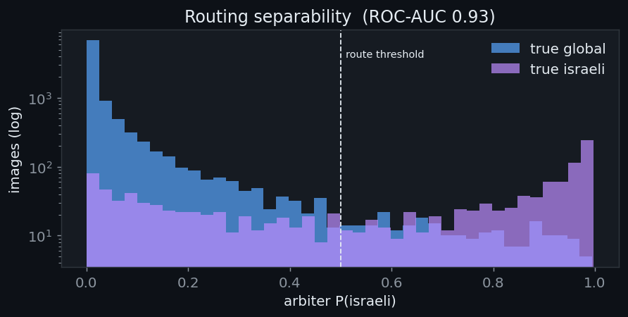
How decisively the arbiter separates the two domains
How to read this chart. For every test image the arbiter outputs one number: P(israeli), its
estimated probability that the image belongs to the Israeli expert (0 on the left, 1 on the right).
The histogram counts how many images fall at each value, on a log scale. Blue bars are images
that are truly global, purple are truly Israeli. A good arbiter pushes blue to the left (low
P) and purple to the right (high P). The dashed line at 0.5 is the decision threshold: anything to
its right is sent to the Israeli model. The clean separation (blue piled near 0, purple piled near 1)
is what a 0.93 ROC-AUC looks like; the small amount of blue and purple that overlap in the middle is
exactly the routing the arbiter cannot get perfectly right. (This histogram illustrates the V1 arbiter;
V2's i_p_background feature sharpened the separation further, lifting AUC to 0.973 and
shrinking that middle overlap.)
Case study: the sufganiyah vs donuts confusion, solved
At the previous review this pair was one of the worst failures in the whole system. A sufganiyah (Israeli jam doughnut) and an American donut look almost identical, and the old single-model setup constantly mixed them up. The two-expert split plus a clean visual cue fixed it.
| Class | Then accuracy | Now accuracy | Confusion with the other |
|---|---|---|---|
| sufganiyah | 58.3% | 88.9% | 82 images read as donuts then → only 2 now |
| donuts | 77.3% | 91.3% | improved, only 5 read as sufganiyah now |
Source: old confusion from FINAL_REPORT_v3_results.csv, current from
datasets/system_evaluation.csv (test split). This is a concrete lesson from the prior
tests carried into the final model, exactly the kind of improvement the review asked us to surface.
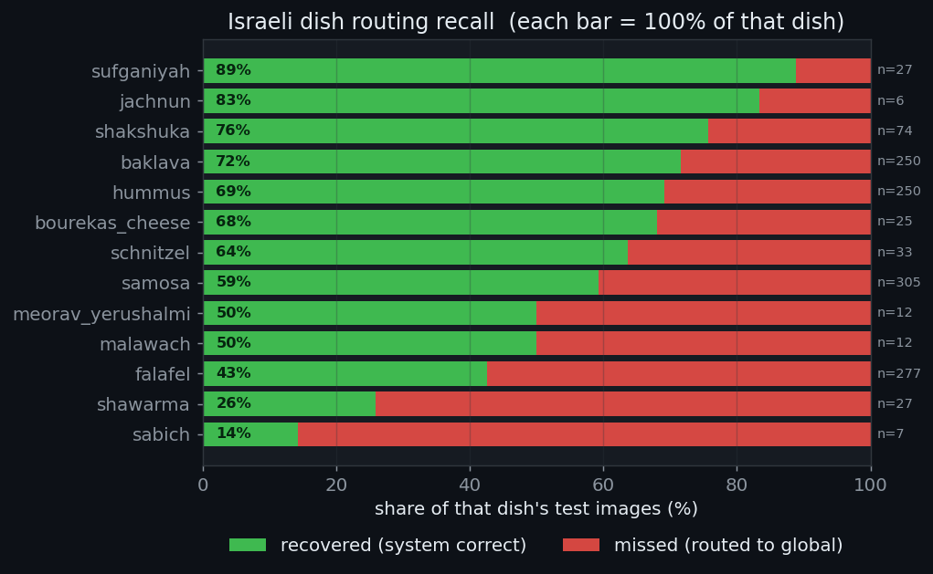
Where the arbiter still misses
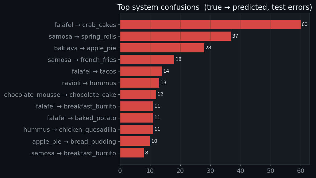
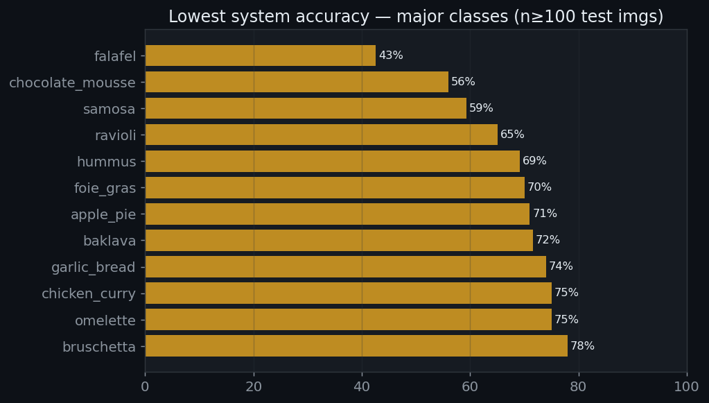
It handles most Israeli dishes well (sufganiyah 89%, jachnun 83%, shakshuka 76%, baklava 72%, hummus 69%) but struggles where a dish strongly resembles a global food: sabich 14%, shawarma 26%, falafel 43%. The dominant single confusion is falafel → crab_cakes (60 images). The limiting factor is visual feature overlap, not the arbiter logic.
Validation Plan and Risk Coverage
Risk → test → evidence
| Risk | Test performed | Evidence / result |
|---|---|---|
| Test accuracy is inflated by data leakage | Recompute val and test top-1 after SHA-1 + perceptual de-dup; compare the two | val 88.16 vs test 88.18 (gap 0.02). Leakage removed |
| Adding local food breaks the global model (catastrophic forgetting) | Compare combined-model accuracy against the two-expert split | Two-expert split keeps global at 88.18% with no degradation |
| The arbiter defaults to one model instead of truly deciding | Count arbiter decisions and measure per-domain recall and ROC-AUC | V2: Israeli recall 79%, global recall 98%, ROC-AUC 0.973; +8.8 pts over always-global (was 61% / 0.93 in V1) |
| A wrong food identification goes unnoticed | Per-image error decomposition into routing error vs both-wrong; per-class recall | 4.91% routing / 11.34% both-wrong, every class measured (System Analysis tab) |
| Class imbalance silently hurts rare classes | Per-class recall reported, smallest classes flagged | Effect confined to ingredient classes with n≈8; reported, not hidden |
| Weight from vision volume is unreliable | Volume estimates validated against Archimedes water displacement | Volume to mass fails on density even when volume is right; pivot to BLE |
| Scale reading is fragile (OCR glare) | Compare OCR of the LCD against direct BLE packet decoding | BLE is deterministic and glare-free; selected as final |
Product vs engineering validation
| Type | What was validated | How |
|---|---|---|
| Engineering validation | Each model and the arbiter meet their numeric targets on held-out, leakage-free data | Held-out test split, ROC-AUC, error decomposition, confusion matrices |
| Product validation | The end user gets a correct food name and weight without manual entry | End-to-end run: photo → class → BLE grams → USDA kcal/macros in the GUI |
Weight estimation: approaches measured and rejected
| Approach | Principle | Why rejected |
|---|---|---|
| Coin fiducial + HoughCircles | ₪1 coin (18 mm) detected, pixels to cm scale | Calibrates the 2-D plane only; no object height |
| MiDaS depth | Monocular relative depth integrated to volume | Scale-ambiguous, noisy on small objects, needs a fiducial every shot |
| Shadow geometry | height = L_shadow · tan(α) | Depends on a known light angle; lighting-sensitive |
| Volume → mass | mass = volume · density | Density problem: fluffy and dense foods of equal volume differ greatly |
| OCR of scale display | Read the 7-segment readout | Glare, angle and lighting fragility on the LCD |
| BLE (final) | Read the weight packet at the source | Selected: deterministic, robust, no vision error |
BLE packet format: weight = low_byte + high_byte × 256, verified by a
checksum over bytes 2 to 6. Example: AC 05 00 02 14 00 CE E4 decodes to 532 g.
The full reverse-engineering story is in the BLE Scale tab.
Reverse-Engineering the BLE Scale
The weight is read straight off the scale's Bluetooth Low Energy broadcast, so there is no camera, no OCR, and no vision error in the measurement path. The scale is a generic commercial unit with no public protocol, so we recovered the packet format ourselves. This tab documents how.
Step 1 · Find the device
Using the nRF Connect app on a phone, we scanned for nearby BLE advertisers. The scale shows up only under a generic name, so we identified it by signal strength (RSSI): with the phone held against the scale, the correct device is the one whose RSSI jumps toward 0 dBm while every other advertiser stays weak. Stepping away and watching that one value drop confirmed the match.
The device advertises as SWAN and streams weight on the notify characteristic
0000ffb2-0000-1000-8000-00805f9b34fb. Subscribing to it delivers a fresh 8-byte packet
every time the reading changes.
Step 2 · Make it talk by changing the input
With the notifications logging, we treated the scale as a black box and changed one variable at a time: place a known mass, record the packet; change the mass, record again. The bytes that moved with weight, and the way they moved, revealed the encoding.
| Mass on scale | Notify packet (hex) | Byte that changed | Decoded |
|---|---|---|---|
| 0 g | AC 05 00 00 00 00 .. | baseline | 0 |
| 100 g | AC 05 00 00 64 00 .. | byte 4 = 0x64 | 100 |
| 200 g | AC 05 00 00 C8 00 .. | byte 4 = 0xC8 | 200 |
| 255 g | AC 05 00 00 FF 00 .. | byte 4 maxed (0xFF) | 255 |
| 532 g | AC 05 00 02 14 00 .. | byte 4 rolled over, byte carries the 256s | 532 |
Step 3 · The packet layout we recovered
| Byte | 0 | 1 | 2 | 3 | 4 | 5 | 6 | 7 |
|---|---|---|---|---|---|---|---|---|
| Role | header | len | unit | status + high bits | low byte | high byte | magic | checksum |
| Example | AC | 05 | 00 | 02 | 14 | 00 | CE | E4 |
low  = packet[4]                          # grams 0..255
high = packet[5] | packet[3]               # number of 256s (carry sits in byte 3)
weight = low + high * 256                  # little-endian, grams
Worked example for AC 05 00 02 14 00 CE E4: low = 0x14 = 20, high =
0x00 | 0x02 = 2, weight = 20 + 2 × 256 = 532 g.
& 0xFE, on the theory that byte 3's low bit was a status flag. It was not: that
bit is the lowest bit of the high byte. Masking it silently dropped 256 g from every odd multiple
of 256, so 272 g read as 16 g while even weights like 532 g looked fine. The fix is to use the full
high byte (no mask). Lesson: never assume a bit is a flag without testing the value range that exercises it.Step 4 · Robust decode in software (a lesson from a real bug)
A live scale flickers as it settles, and the high byte can momentarily read wrong during a refresh, which would make a 532 g reading drop to 20 g for one frame. Our first attempt held the high byte with a sticky latch. That was a mistake: a single transient overshoot (pressing down so it briefly reads above 255 g) latched a permanent +256 g offset that never cleared, so a load removed and replaced read double (200 g, then 400 g). The latch also refused to return to 0 if the scale stopped sending a clean zero packet.
from bleak import BleakScanner, BleakClient
from collections import deque
NOTIFY_UUID = "0000ffb2-0000-1000-8000-00805f9b34fb"
raw = deque(maxlen=5)

def on_notify(sender, data):
    b = list(data)
    if len(b) < 8: return
    low  = b[4]
    high = b[5] | b[3]                   # full high byte, no mask (see odd-256 bug)
    raw.append(low + high * 256)
    weight = sorted(raw)[len(raw) // 2]   # median: no latch, returns to 0, rejects spikes
    # ... push to UI, mark STABLE when last 10 samples vary ≤ 2 g

async def run():
    dev = await BleakScanner.find_device_by_name("SWAN")
    async with BleakClient(dev) as c:
        await c.start_notify(NOTIFY_UUID, on_notify)
The weight-calculation state machine (per packet)
Every notification runs through the same fixed pipeline before it becomes a gram value shown to the user. This is the state machine that computes the weight: validate → decode → median → calibrate → stability → emit. A frame that fails validation is dropped, not shown.
| Stage | Computation | Output |
|---|---|---|
| Validate | len≥8, header ==0xAC, sum(b[2..6])&0xFF==b[7] | pass, or drop |
| Decode | low=b[4]; high=b[5]|b[3]; raw=low+high*256 | raw grams |
| Median | median of the last 5 raw values | flicker-free grams |
| Calibrate | g = round(1.178 × median) (through-origin span fix) | true grams |
| Stability | max−min of last 10 g ≤ 2 g ? | STABLE / MOVING |
| Emit | current_weight = g | value used for calories |
food_app.py), but it was fragile to glare and viewing angle, and
every vision volume method failed on the volume-to-mass density problem (see the
Validation & Risks tab). BLE removes the
measurement from the vision path entirely. Source: gui_scale.py, used live in
DEMO.py.Step 4b · Calibrating the scale: from a 16% span error to a specified instrument
A digital scale is only trustworthy if its reading matches true mass, and calories scale linearly with weight, so any weight error passes straight into the calorie figure. Testing this BLE scale against reference masses exposed a fault: it read a steady ~16% low across the whole range. Crucially the error was systematic, not random: repeated placements of the same mass agreed to within a few grams, which means it is a multiplicative span error, and systematic errors are correctable in software.
The experiment. Ten reference masses from 21 g to 1062 g (water measured on an accurate
scale) were each read five times on the scale's own LCD, at a fixed centred placement (a spreader
plate removes the single-load-cell eccentricity effect). To test that the fit generalises rather
than curve-fitting water, we then measured ten completely different everyday objects (phone,
battery, glass, remote, cardboard, camera, toys) as a held-out validation set. Both are
plotted below: blue = fit set,
amber = held-out objects. A perfect scale would lie on the dashed
y = x line; every point sits above it, because the scale reads low, and it does
so by a constant proportion - which is why both sets fall on the same straight line through
the origin.
The regression (exactly what we computed). We want a correction that maps each raw reading
ŷ onto the true mass. Every candidate is scored by its mean absolute error (MAE)
over the n = 10 reference masses - the average gap between the corrected reading and the truth:
We fit two candidates to the same 10 masses by least squares and compared their MAE:
| Model | Equation | Fitted numbers | MAE | Max error |
|---|---|---|---|---|
| No correction (raw) | ŷ = raw | none | 50.7 g (16.1%) | 150 g |
| Two-parameter line | ŷ = a + b·raw | a = +2.846 g, b = 1.1728 | 4.9 g | 12.7 g |
| Through-origin (shipped) | ŷ = k·raw | k = 1.17804 | 5.1 g | 12.5 g |
The two fitted models are tied on error (4.9 vs 5.1 g), but the two-parameter line carries a
spurious +2.846 g intercept that over-reads light items (it would turn a true 0 g into 2.85 g,
and a 53 g portion into 64 g). A load-cell span error is physically multiplicative, so the honest
model is forced through the origin (a = 0), and its single gain k is the
least-squares through-origin slope - literally the two sums from our data divided:
The result. The correction collapses the error from a 16% span to a flat few grams across the entire range. The chart below shows absolute error before and after: the raw error grows linearly with load (the signature of a span error, reaching 150 g at 1 kg), while the corrected error stays near zero and no longer trends with mass.
Formula output vs the truth (the whole calibration in one picture). The most honest way to
show the engineering is to plot, for every object, three numbers at once: the
raw reading the scale actually gave (before any software touched
it), the exact output of our formula 1.178 × raw,
and the true weight (the dashed diagonal, where reading = truth). The raw readings sit
visibly below the diagonal - the scale under-reports - while the formula output lands
on it. This is measured, corrected, and verified against ground truth in a single view: it is
a real correction of a physical instrument, not a number we invented.
Zoomed to the light end (0 to 130 g). On the full-range plot above the lightest items are crushed into the corner, so here is the same data zoomed in. Even a 5 g object follows the exact same relationship - raw below the truth, formula output on it - and the 3 g item is the dead-zone case: the scale reads 0, so both the raw point and the formula output sit on the axis while the true weight is 3 g (no multiplicative fix can lift a zero).
| Reference | True (g) | Mean raw (g) | Raw error | Corrected = 1.178×raw | Corrected error |
|---|---|---|---|---|---|
| low_20 | 21 | 15.8 | −5.2 (24.8%) | 19 | −2 (9.5%) |
| low_50 | 29 | 25.4 | −3.6 (12.4%) | 30 | +1 (3.4%) |
| low_100 | 95 | 81.0 | −14.0 (14.7%) | 95 | 0 (0.0%) |
| low_150 | 154 | 135.0 | −19.0 (12.3%) | 159 | +5 (3.2%) |
| tuna | 162 | 133.6 | −28.4 (17.5%) | 157 | −5 (3.1%) |
| yogurt | 209 | 175.0 | −34.0 (16.3%) | 206 | −3 (1.4%) |
| water_362 | 362 | 301.6 | −60.4 (16.7%) | 355 | −7 (1.9%) |
| water_477 | 477 | 401.8 | −75.2 (15.8%) | 473 | −4 (0.8%) |
| water_708 | 708 | 590.4 | −117.6 (16.6%) | 695 | −13 (1.8%) |
| water_1062 | 1062 | 912.0 | −150.0 (14.1%) | 1074 | +12 (1.1%) |
Held-out validation: the water-fit constant generalises to unseen objects
The constant above was fit on water and food only. To prove it captures the scale's true
physical span error rather than a water-specific curve, we applied the unchanged
k = 1.178 to ten objects it never saw - a phone, a battery, a drinking glass, a remote,
cardboard, a camera and some toys. It predicts their true mass to a mean absolute error of just
1.9 g (mostly within ±1-3%), across metals, glass, plastic and card. This is a genuine
generalisation test, and refitting the slope on all 20 objects barely moves it
(1.17804 → 1.17825), so the shipped constant is left unchanged.
| Held-out object | True (g) | Mean raw (g) | Corrected = 1.178×raw | Error |
|---|---|---|---|---|
| tiny screwdriver | 3 | 0.0 | 0 | −3 (below detection floor) |
| tiny screwdriver ×2 | 5 | 4.2 | 5 | 0 (0%) |
| ball toy | 23 | 20.6 | 24 | +1 (+4.3%) |
| carrot toy | 44 | 37.6 | 44 | 0 (0%) |
| cardboard | 47 | 38.6 | 45 | −2 (−4.3%) |
| camera | 116 | 100.2 | 118 | +2 (+1.7%) |
| remote | 123 | 103.0 | 121 | −2 (−1.6%) |
| battery | 224 | 194.2 | 229 | +5 (+2.2%) |
| phone | 241 | 202.4 | 238 | −3 (−1.2%) |
| drinking glass | 289 | 242.6 | 286 | −3 (−1.0%) |
1.178 × 0 = 0).
Doubling it to 5 g was detected correctly. The honest specification is therefore a practical lower
limit of ~5 g: below it the weight (and any calorie figure derived from it) is unreliable. This
matters only for near-weightless items (a pinch of spice, a single sweet) and is surfaced as a
limitation rather than hidden.- Shipped formula (identical in the desktop demo, the ONNX edge exe, and the browser app):
corrected_g = 1.178 × raw, applied right after the 5-sample median filter; the reverse-engineered byte decode is left untouched. - Validated on 20 objects (10 fit + 10 held-out): mean absolute error 3.6 g after correction, down from 34.0 g (16-20%) raw. On the held-out objects alone the error is 1.9 g, confirming the constant generalises rather than curve-fitting the training set.
- Max error ≈ ±13 g over the full 5 to 1062 g range; as a fraction this is best mid-range (~1 to 3%) and only the smallest masses show a larger percentage (a few grams on a 20 g item).
- Lower limit ~5 g: below a ~4 g detection floor the scale reads exactly 0 and cannot be
corrected. The slope itself is stable (
k = 1.178, unchanged when refit on all 20). - The residual is now dominated by the scale's own repeatability (mean spread ~10 g, up to 31 g at 1 kg), not by the fit: the correction has reached the hardware noise floor, and the median filter smooths what remains.
- This is why the app deliberately shows a different number than the scale's LCD: the LCD shows
the uncorrected raw value; the app shows calibrated true mass. Source data:
scripts/eval/weights_cal.csv, fit byscripts/eval/weight_calibration.py.
Step 5 · The connection state machine
The BLE driver is a finite state machine: it discovers the scale, subscribes, streams and
decodes packets, judges stability, and self-heals if the stream goes silent. Every packet is
validated (length ≥ 8, AC header, and the additive checksum over bytes 2..6) before it
is decoded, so a corrupt frame is dropped rather than shown.
| State | Event | Action | Next state |
|---|---|---|---|
| DISCONNECTED | user connects | start BLE scan | SCANNING |
| SCANNING | advertiser SWAN / strongest RSSI | open GATT connection | CONNECTING |
| CONNECTING | GATT connected | enable notifications on ffb2 | SUBSCRIBING |
| SUBSCRIBING | notify enabled | start the packet loop | STREAMING (MOVING) |
| STREAMING | valid packet | decode, push to 5-sample median | MOVING or STABLE |
| STREAMING | bad header / length / checksum | drop the frame | STREAMING (no change) |
| MOVING | last 10 samples vary ≤ 2 g | latch a reading as settled | STABLE |
| STABLE | a later sample varies > 2 g | reading is moving again | MOVING |
| STREAMING | no packet for > 4 s (watchdog) | tear down and re-scan | STALE → CONNECTING |
| any | GATT disconnect | reset weight to 0 | DISCONNECTED |
Live Demo: the End-to-End Application
The demo ties everything together: a webcam frame becomes a food class, a BLE weight,
and a full nutrition breakdown, live. It runs the current Global and Israeli models behind the
XGBoost arbiter, with a Gemini vision fallback for the cases the experts cannot handle. Every design
choice below is made for one goal: a correct result in the room, under any camera and any light, as
often as the score promises. Source: scripts/demo/caleyez_demo.py.
scripts/demo/onnx_backend.py) feeds the arbiter the identical features, so routing is
unchanged. We verified the ONNX models match the PyTorch ones to 0% top-1 mismatch on 200 test images
per model, and the full pipeline (two ONNX models + the XGBoost arbiter) agrees on the routing
decision for every image (max ΔP(israeli) = 0.013). Measured inference is
~0.35 s per analysis on a CPU (versus ~1-3 s for the PyTorch-CPU build), in a much
smaller, torch-free executable. PyInstaller then packages it into a single standalone .exe
with the ONNX models bundled inside - copy the folder to any Windows laptop and run it. Build:
build_edge_onnx/.The pipeline per capture
Preprocessing, step by step (animated)
This is exactly what happens to the pixels between the webcam and the network. Press play to watch one frame travel through the four preprocessing stages and into both experts.
| Stage | What happens | Why |
|---|---|---|
| 1 · Center ROI crop | Crop the central square of the frame (the green "place food here" box, about 60% of the short side). | Deterministic and scale-consistent: the food fills a known fraction on every camera, with no silent failures. Replaces the old idea of auto-detecting a plate. |
| 2 · Letterbox to imgsz | Resize the square to the model input size (320 for Global, 224 for Israeli) inside Ultralytics predict(). | The model always receives the exact geometry it trained on, so a 720p and a 4K camera produce the same tensor. No aspect-ratio distortion. |
| 3 · Normalise | Pixel values are scaled from 0..255 to 0..1 (the network's expected range). | Matches training preprocessing exactly. |
| 4 · Into both experts | The same tensor is classified by the Global and Israeli models in a single forward pass each. | One predict() per model, identical to how the arbiter's training features were generated, so routing behaves exactly as evaluated. |
What we deliberately do NOT do (lessons from testing)
The preprocessing is intentionally minimal. Several "smart" steps were tried and then removed because measurement showed they hurt. Keeping the record is the honest engineering story.
| Tried | Measured effect | Decision |
|---|---|---|
| Gray-world white balance | Desaturated dominant-colour foods (a red pepper read as a beige pastry), because gray-world assumes the scene averages to neutral gray. | Removed |
| GrabCut food segmentation | On a clean hummus image the prediction dropped from 96% to 92% wrong (malawach). The models are already background-robust (a pepper scores 99.97% on a dark or wood background), so segmenting was pure harm. | Removed |
| CLAHE + test-time averaging | Averaging raw and CLAHE softmaxes shifted the confidence values away from the distribution the arbiter was trained on, which broke routing (confident Israeli dishes were sent to the Global model). | Removed |
Why a fixed center ROI
The crop is a fixed central square (the on-screen guide box), not an automatically detected plate.
| Approach | Behaviour | Verdict |
|---|---|---|
| Automatic (HoughCircles / GrabCut / contours) | Depends on a clean plate, even light and a plain background; fails silently on clutter and returns a wrong crop (measured: it broke clean predictions). | Unpredictable on stage |
| Fixed center ROI (chosen) | A drawn "place food here" box; we always crop that square. | Deterministic, scale-consistent, no silent failures |
The deeper finding: camera angle, not background
Testing exposed something more fundamental than clutter. The Global model classifies a bell pepper at 99.97% even when it fills only a quarter of a dark-scale or wood background, so background and crop size are not what break it. What breaks it is the viewing angle: the training images are almost all side or eye-level views, while a top-down demo camera sees a red disc with a central stem, which is genuinely out of distribution and can read as chocolate cake.
Wiring the real arbiter (not a re-implementation)
The demo runs the V2 Israeli model (14 classes: the 13 dishes plus background) and
computes the same 20 features the arbiter was trained on, in the same order, then loads the exact
saved model. The 20th feature is i_p_background, the Israeli model's "this is not one of my
dishes" probability, which is now the arbiter's single most important feature.
g = expert(global_model, roi, imgsz=320)   # top-5 conf, entropy, margin
i = expert(israeli_model_v2, roi, imgsz=224) # also reads P(background)
X = [g_conf1..5, g_entropy, g_margin,
     i_conf1..5, i_entropy, i_margin, i_p_background,
     conf_gap, conf_ratio, entropy_gap, margin_gap, both_unsure]
p_israeli = arbiter.predict_proba(X)[1]     # scripts/arbiter/arbiter_xgb.json (V2, 20 feats)
route_to_israeli = p_israeli >= 0.5
background, the demo
treats that as an abstain and falls back (never showing "background" as a food). The decision panel
shows both experts' top guess, the live P(israeli), and the per-feature contributions, so routing is
visible, not hidden.The Gemini fallback: covering the cases no expert can win
About 11% of system errors are images where both experts are wrong (the both-wrong pool from the System Analysis tab). No amount of routing fixes those. The demo detects that situation and asks a cloud vision model instead, which is the honest way to push realized accuracy past the local ceiling on hard inputs.
| Trigger | Condition | Meaning |
|---|---|---|
| Weak chosen expert | chosen top-1 below its gate (0.55 global, 0.60 Israeli) | The selected model is not confident enough to trust |
| Both experts unsure | both top-1 below 0.50 (both_unsure) | The input is likely out of both label spaces |
| Arbiter undecided | P(israeli) within 0.15 of 0.50 (ARBITER_BAND) | The router cannot confidently pick an expert |
| Israeli abstains | routed to Israeli but its top-1 is background | The Israeli model says "not my dish" -> defer instead of forcing a label |
The two gates differ on purpose: the Global model spreads probability over 132 classes, so a modest top-1 is still meaningful, while the Israeli model has only 13 classes and must clear a higher bar to be believed. When either trigger fires, the ROI crop is sent to Gemini and its label drives the nutrition lookup. The UI marks these results so the source is never ambiguous.
UI and UX choices
| Choice | Why |
|---|---|
| Tkinter desktop app | The system is an edge device: models, camera and BLE all run locally with no server. Tkinter ships with Python, starts instantly, and binds cleanly to the OpenCV camera loop and the BLE thread, which a browser UI cannot do without extra bridges. |
| Live decision panel | Two confidence bars (Global, Israeli) plus the live P(israeli) make the routing visible while you demo. The reviewer point that the router was unclear is answered on screen: you watch it decide. |
| "Why" force chart (TreeSHAP) | For each capture the panel draws the exact per-feature contributions to the routing decision (bars pushing toward Global or Israeli), computed with TreeSHAP from the XGBoost arbiter. The decision is not just shown, it is explained on the spot. |
| Data-tagging flywheel | Type the true dish (autocompleted from all 145 class names) and every capture is logged: the cropped image (training-ready), both 512-D embeddings, and a verification row with each model's prediction and correctness. Demo failures become labelled fine-tuning data. |
| Embedded interactive log, not popups | The day's meals live in a table inside the main window with running calorie and macro totals, colour-coded by which expert produced each row (blue global, teal Israeli). Add and delete update in place, so logging is part of the flow rather than a separate dialog. |
| Threaded inference | Inference runs on a worker thread so the camera preview and weight readout never freeze while the models think. |
| Weight colour state | The big weight readout turns teal only when the BLE stream is stable (last ten samples within 2 g), so you capture on a settled reading, not a bouncing one. |
| Manual weight fallback | If the BLE scale is not connected, a small "manual g" field is used automatically, so a flaky Bluetooth link can never block the demo. The app states which source is live. |
| API keys from the environment | USDA and Gemini keys are read from environment variables, never hard-coded, so the public repo carries no secrets. |
scripts/demo/caleyez_demo.py.The Web App: Edge AI in the Browser
The same two-expert pipeline that runs on the desktop also runs, unchanged, inside a phone
browser - no install, no app store, no server doing the inference. A judge scans a QR code and the
two CNNs plus the XGBoost arbiter execute on their own device. This tab documents how a browser becomes an
edge-AI runtime, how it uses the device's CPU/GPU and memory, where the cloud is and is not used, and the
hard limits of the platform. Repo: caleyez-web (public, GitHub Pages). Live:
raz-dv-ee.github.io/caleyez-web
· engineering console: /engineering.html · latency bench: /bench.html.
⚡ N ms
    · on-device edge
) next to every result, so there is no hidden HTTP round-trip to explain.How a browser runs a neural network on the edge
The two YOLO11l-cls experts are exported to ONNX (the same models the desktop ONNX build uses) and
executed with ONNX Runtime Web (onnxruntime-web). ORT-Web ships the runtime as
a WebAssembly (WASM) module, so the network's operators run as near-native compiled code inside the
browser sandbox - this is what makes real CNN inference on a phone practical rather than a toy.
| Backend | What it uses | When | Trade-off |
|---|---|---|---|
| WASM (default) | the device CPU, SIMD, single-threaded | always, unless opted out | Widens the fp16 weights to fp32 at run time, so it makes the same top-1 decision as desktop (only ~10−3 probability drift). Chosen as default. |
WebGPU (?gpu=1) | the device GPU, fp16 compute | opt-in via URL | Faster steady-state, but a ~2.6 s one-time shader compile (hidden behind the loading splash) and fp16 rounding degraded a few classes on some mobile GPUs - so it is not the default. |
?gpu=1.fp16 vs fp32, and why it matters here
A neural network is millions of numbers (the weights). fp32 ("single precision") stores each weight as a 32-bit floating-point number; fp16 ("half precision") stores it in 16 bits. Half the bits means half the memory and faster movement through the processor, but lower numeric precision: fp16 can represent far fewer distinct values, so very small differences get rounded away. We publish the models in fp16 so each download is roughly half the size (about 25 MB instead of about 50 MB) and they sit comfortably in phone memory. The two backends then treat those fp16 weights differently, and that is the crux of our default:
| fp32 (single precision) | fp16 (half precision) | |
|---|---|---|
| Bits per weight | 32 | 16 |
| Size / memory | baseline | about half |
| Numeric precision | full | lower (more rounding) |
| In CalEyeZ | WASM widens fp16 to fp32 before computing, so the arithmetic stays full precision and makes the same top-1 decision as desktop (~10−3 probability drift, not bit-identical) | WebGPU computes directly in fp16: faster, but the rounding can flip a borderline prediction |
So the phone downloads small fp16 files either way; on the default CPU path each weight is widened to fp32 for the computation. Widening does not recover the bits fp16 dropped - a widened fp16 value is the same rounded number with trailing zeros, no new information - it just stops the millions of multiply-adds from re-rounding at every step, which is where fp16 compute actually loses accuracy. The only difference left from desktop is a ~10−3 probability drift from rounding the weights to fp16 once at export; the decision is identical. That single distinction is why CPU/WASM is the default and WebGPU is opt-in.
1000 + 0.04 = 1000
(the 0.04 is below its precision, so it vanishes); do that a hundred times and you still read 1000
when the truth is 1004. The 8-digit calculator keeps 1000.0400 → 1004.0000.
So fp16 arithmetic quietly drops small activations that can decide a borderline food. Widening to fp32 loads
the same 4-digit weight into an 8-digit register so every step afterward has room - the zeros are just the
loading; the win is the arithmetic. The desktop uses the same 8-digit (fp32) arithmetic, which is why the browser
matches its decision; the only residual gap is 4-digit vs 8-digit inputs (~10−3),
which never piles up. “Just compute in fp16” means doing every step on the 4-digit calculator, so the
rounding compounds thousands of times - and that is what flips pizza vs hamburger on the WebGPU path.What a “mantissa” is, and the multiply that overflows it
A floating-point number is stored as sign × mantissa × 2exponent. The mantissa holds the significant digits, and the number of mantissa bits is what sets the precision. fp16 has 10 mantissa bits (~3-4 decimal digits); fp32 has 23 (~7 digits). The exponent handles magnitude, so fp16 isn’t short on range (it reaches 65,504) - it’s short on digits. That is the “room to grow” you need: not room for bigger numbers, room for more significant digits.
Watch it in one multiply-accumulate - the operation a CNN does millions of times. Multiply a weight by an activation, each stored to ~4 digits (fp16):
weight 1.234  ×  activation 5.678  =  7.006652   ← the exact product needs 7 digits
   fp16 (10-bit mantissa) → rounds back to 7.007     ← the tail .000652 is chopped
   fp32 (23-bit mantissa) → keeps       7.006652     ← all 7 digits fit
In bits: two 10-bit mantissas multiply into a result up to ~20 bits wide - fp32’s 23-bit mantissa has room to hold it, fp16’s 10-bit does not, so fp16 rounds it away at every step. That is exactly your intuition - the product of two 16-bit numbers wants ~32 bits, and only fp32 keeps them. A layer sums thousands of these products, so in fp16 the chopped tails compound; in fp32 they stay. Widening the fp16 weights to fp32 before computing gives each intermediate product that room - which is the whole point of computing at higher precision than you store.
z = Σ w·x inherits that: worst case ~5×10⁻⁴, usually
less (random errors cancel). (3) Softmax passes it through ~1:1 - e.g. top logit 8.000 vs runner-up 6.000 gives
p = 1/(1+e−2.000) = 0.88080; nudge the margin to 2.004 and
p = 0.88121 - a 4×10⁻⁴ shift. The measured max over all
rows/classes is ~10−3. The top-1 only flips if the two best probabilities sit within
10−3 of each other; real margins are ~0.1+ (0.88 vs 0.12), so it never crosses - which is why
the parity test found 0 top-1 mismatches.One weight, followed end to end
The whole story on a single number - how an fp32 weight is cut to fp16, padded with zeros, and how the calculation refills those zeros and still lands on the same answer as the full model:
0.71341827 (fp32) → stored as
0.7134 (fp16). The low digits …1827 are dropped for good - the only
precision ever lost.2 · Widened in memory (at load). to compute,
0.7134 goes into a 32-bit slot as
0.71340000 - the freed low bits are filled with
zeros. No information added; still 0.7134.3 · The arithmetic fills the zeros. multiply by an activation
0.8207:
0.7134 × 0.8207 = 0.58548738 - the new digits
8738 land exactly in the slots that were zero. fp16 re-rounds them away
(0.5855); fp32 keeps them.4 · The numbers drive the logit. a neuron sums thousands of such products; keeping those tails (fp32) instead of chopping them every step (fp16) makes the summed logit match the full model - here
8.004 vs the full-fp32 model's 8.000.5 · Same decision; drift blown away. softmax vs a runner-up logit
6.000:
P = 1/(1+e−2.004) = 0.88121 vs the full model's 0.88080 - a
4×10⁻⁴ gap. The winner leads by tenths (0.88 vs 0.12), so a
10−3 nudge can't cross it.
So the light fp16-shipped model reaches the identical decision as the heavy fp32 model - the only thing that differs is the third decimal of the probability, which never decides an answer. That is why we can ship the small file and still be desktop-exact where it counts.
The options we actually weighed
Two independent choices: what format to ship the file in, and what precision to do the math in. Here is every end-to-end option and what it would cost:
| Option (ship → compute) | Download | Accuracy | Speed | Verdict |
|---|---|---|---|---|
| fp32 file → fp32 math | ~100 MB | the full-precision reference | CPU, ~0.6 s | Rejected: doubles the download for no visible gain - it ends up computing in fp32 anyway (same RAM), and the fp16 version already reaches the identical decision. |
| fp16 file → fp32 math (chosen, default) | ~50 MB | same top-1 decision (~10−3 drift) | CPU, ~0.6 s | Chosen: half the download, desktop-identical decisions. Widening to fp32 is free and keeps the arithmetic clean. |
| fp16 file → fp16 math (WebGPU, opt-in) | ~50 MB | can flip borderline foods | GPU, fastest | Opt-in only: fp16 compute accumulates rounding; it flipped pizza/hamburger on some mobile GPUs. Behind ?gpu=1 for benchmarking. |
| int8 file (quantized) | ~25 MB | too coarse for food texture | fast | Rejected: 8-bit steps are too coarse and flip the subtle textures that separate look-alike dishes. |
Memory and CPU: what the phone actually does
Two fp16 ONNX models are downloaded once: Global ≈25 MB (320², 132 classes) and Israeli ≈25 MB (224², 13 classes + background) - ≈50 MB total, then HTTP-cached so later runs are instant. At run time WASM upcasts fp16→fp32, so a few hundred MB of working memory is touched during inference; the app targets devices with ≥2 GB RAM.
The CPU matters as much as the memory. Because the default path runs on WebAssembly, the actual matrix maths happens on the phone's CPU, so the processor's speed sets the inference time directly: a recent flagship CPU finishes both models in about 0.6 s, while an older or budget CPU is proportionally slower for the exact same work. This is why the models are sized deliberately (fp16 weights, 320/224 inputs, single-threaded WASM) to stay interactive on mid-range phones rather than only flagships, and why the app prints the measured time on every result so the device's real capability is visible rather than assumed. A phone with plenty of RAM but a weak CPU will still run correctly, just with a longer wait per photo.
dispose(tg,ti,go,io)); without this the heap would grow with every photo and eventually
crash the tab - the risk is largest on the WebGPU path where output tensors hold GPU buffers. A one-shot
warm-up inference on load also compiles the kernels ahead of the first real photo, so the cold-start
cost is paid behind the splash, not in front of a judge.
Bit-for-bit pipeline parity with the desktop
The browser preprocessing is written to match scripts/demo/onnx_backend.py so the two runtimes
agree on the answer. Central ROI square (0.60) → resized on a canvas to each model's input
(imageSmoothingQuality:'high') → ÷255, RGB, CHW, and no ImageNet
normalisation (the ÷255 is the only scaling - verified on the desktop as the exact
preprocessing). This was validated at 0% top-1 mismatch against the reference pipeline.
| image-processing step | worked example | |
|---|---|---|
| 1 | capture source frame | 1920 × 1080 px |
| 2 | centre-crop ROI (60%), discard the outer 40% (plate / background) | 648 × 648 px at (636, 216) |
| 3 | resample to each model's input (bilinear, high quality) | → 320 × 320 and 224 × 224 |
| 4 | read RGBA bytes, drop alpha → RGB (0-255) | a pixel = (183, 92, 47) |
| 5 | normalise ÷255: byte → float in [0, 1] | (183, 92, 47) → (0.718, 0.361, 0.184) |
| 6 | pack HWC → CHW planar tensor | [1, 3, 320, 320] |
| 7 | verify range over the whole tensor | min / max / mean all in [0, 1] |
The XGBoost arbiter, re-implemented in JavaScript
ORT-Web has no TreeEnsemble operator, so the router cannot run as ONNX in the browser. We instead
export the trained booster to a flat JSON (arbiter_trees.json) and walk the trees in JavaScript.
This is copying, not retraining, and not an approximation - and below is exactly how, in plain terms.
The math (two lines)
1. Add the votes. Each tree fk sends the 20-feature vector x to one
leaf and returns that leaf’s vote. Sum the 400 votes plus the base margin b0:
2. Squash to a probability. The sigmoid turns the log-odds score into P(israeli):
That is the entire model - a weighted show of hands, then a sigmoid. Nothing is learned in the browser; the votes and questions were fixed at training time.
Converting it to the browser - 3 mechanical steps
The export script scripts/arbiter/export_arbiter_trees.py does exactly this and nothing more:
- Dump the trees. XGBoost’s own
booster.get_dump("json")writes all 400 trees as JSON (feature, threshold, children, leaf values). - Flatten each node into a tiny array the browser can read: an internal node becomes
[feature#, threshold, go-if-yes, go-if-no]; a leaf becomes[vote]. - Compute the base. The starting number is the log-odds of the overall Israeli rate:
base = ln(p/(1−p))withp = 0.21763562→ −1.2795.
So one node in the file literally reads "0":[14, 0.000047, 1, 2] = “at the root, look at
feature 14 (i_p_background): if it’s below 0.000047 go to node 1, else node 2.”
Walking the file is then a dozen comparisons per tree:
function arbiterP(f){              // f = the 20 features
  let m = ARB.base;                // start at the base log-odds (-1.2795)
  for (const tree of ARB.trees){
    let n = tree["0"];             // root node
    while (n.length > 1)           // length 4 = internal, length 1 = leaf
      n = tree[ Math.fround(f[n[0]]) < n[1] ? n[2] : n[3] ];  // [feature,threshold,yes,no]
    m += n[0];                     // add this tree's vote (the leaf value)
  }
  return 1 / (1 + Math.exp(-m));   // sigmoid -> P(israeli)
}
Math.fround matters (and how we verified it). XGBoost compares in
32-bit floats internally, so the JS casts each feature with Math.fround before the
< threshold test. The export script re-derives arbiter_trees.json from the trained
arbiter_xgb.json and checks it against the Python model on all 32,136 held-out rows: max
probability gap 3.8×10⁻⁷ and 0 routing disagreements. (Without
Math.fround, ~0.08% of borderline routes could differ from the desktop.) The routed probability then
feeds the same gates as desktop (GATE_G 0.55, GATE_I 0.60, both-unsure 0.50, arbiter-band 0.15),
so browser and desktop make the identical call.Latency, measured and shown
Inference is timed with performance.now() around the two run() calls and printed on
the result as ⚡ N ms · on-device edge (and in the engineering console
header). On a Pixel 10 Pro the warm inference is ≈0.6 s for both models + arbiter on
the WASM path. Beyond honesty, this number is a demo argument: a live-updating on-device timer makes it
self-evident that recognition is not a cloud call.
Where the cloud is used (and where it is not)
Recognition is 100% local. Two things legitimately use the network, and both go through a Cloudflare Worker so that the API keys are stored as Worker secrets and never appear in the public web-app repo. The single worker routes by HTTP method: GET = USDA, POST = Gemini.
| Service | Purpose | Why a Worker | Notable engineering |
|---|---|---|---|
| USDA proxy (GET) | nutrition for foods not in the local DB | keeps the free USDA key server-side; 30-day edge cache | Smart filter: rejects junk descriptions (juice/dried/sauce…), scores by primary-name and
token overlap, treats cooking words as stop-words, and penalises ALL-CAPS branded/restaurant entries -
so "apple"→apple, not apple juice, and "grilled salmon"→salmon. ?debug=1 returns the
ranked candidate list for the engineering console. |
| Gemini vision (POST) | identify the food when the on-device system is unsure | keeps the Gemini key server-side; multimodal call | Mirrors the desktop demo's fallback: when the confidence gate / arbiter band says "not sure," the ROI
image is POSTed to gemini-flash-latest with the demo's exact prompt, and the returned food
label overrides the local guess (marked with a 🔮 chip). Also available as a manual override button. |
Cooking method, portion sub-types, and evidence-based calories
Calories change drastically with preparation, so the app offers a cooking-method choice
(raw / boiled / grilled / fried / deep-fried) - but only for foods
where it makes sense (an apple gets no dropdown; a steak does), driven by a per-class metadata file
(foodmeta.json). A steak can also be refined to a specific cut (filet mignon, ribeye…),
each carrying its own curated per-100 g macros.
scripts/eval/cooking_multipliers.py): for
each pair the per-100 g cooked/raw kcal ratio is the multiplier, aggregated with a sample count and 95%
confidence interval. Because the scale weighs the cooked food, per-100 g-cooked is exactly the right
basis. Result: raw ×1.0, boiled ×1.04, grilled ×1.17, fried ×1.47,
deep-fried ×1.99 - each shown in the engineering console with its n and CI.Weighing: the BLE scale in the browser
Portion mass comes from the same reverse-engineered SWAN scale, read over Web Bluetooth: connect to
device SWAN, subscribe to notify characteristic ffb2, and decode the 8-byte packet
(weight = low + (high|carry)×256, additive checksum over bytes 2-6). See the
BLE Scale tab for the full protocol. When no scale is present, grams
are entered manually. Web Bluetooth is Chromium-only, which is the app's sharpest platform limit (below).
The engineering console: the whole pipeline, exposed
/engineering.html is a diagnostic view that traces one capture end to end: the preprocessing
thumbnails, both experts' top-5 with entropy/margin/P(background), the 20-feature arbiter vector, the arbiter
P(israeli) with every gate shown PASS/FAIL, the USDA smart-filter candidate table (scores + reject reasons),
the cooking-multiplier math with n/CI, a live per-byte BLE packet decode with checksum verification, and
a compatibility/requirements section. It exists so the engineering is legible as structured evidence, not a
black box.
Limitations of the browser platform
Running on the open web means the browser and hardware set real limits. These are stated plainly rather than hidden, and are also surfaced in the app's own compatibility section.
| Limit | Cause | Effect / mitigation |
|---|---|---|
| BLE scale is Android-Chrome only | Web Bluetooth is unsupported on iOS (Safari and Chrome-iOS both use WebKit) and Firefox | On iPhone the scale cannot pair → the app falls back to manual grams. Best full experience is Android Chrome. |
| Memory / download | ≈50 MB of models + fp32 upcast at run time | Needs ≥2 GB RAM; very old low-memory phones may struggle. Models cache after first load. |
| CPU speed sets the latency | the default WASM path runs the inference on the phone CPU | A flagship CPU gives about 0.6 s; an older/budget CPU is proportionally slower for the same work. The models are sized (fp16, 320/224 inputs) to stay interactive on mid-range phones, and the measured time is shown on every result. |
| WebGPU accuracy | fp16 compute rounding on some mobile GPUs | Left off by default; CPU/WASM (fp32-accurate) is the default path. |
| Network for nutrition / Gemini | USDA and Gemini are cloud services | Recognition works fully offline after first load; only the nutrition lookup and the "unsure" Gemini fallback need connectivity. |
| Camera needs HTTPS | getUserMedia requires a secure context |
Served over HTTPS via GitHub Pages; fine in practice. |
Hosting architecture
The app repo (caleyez-web) is deliberately tiny - HTML/JS only, no models - so
GitHub Pages deploys it in seconds. The ≈50 MB of ONNX models, the arbiter trees, the class-name
maps, foodmeta.json, and cooking_multipliers.json are hosted in this repo under
/webmodels/ and fetched cross-origin (CORS-enabled) via MODEL_BASE. Keys live only in
the Cloudflare Worker as secrets. Net result: a phone loads a few kB of HTML, pulls the models once from a CDN,
and thereafter runs an entire multi-model food-recognition system locally.
Points Raised in Review and How We Addressed Them
The points raised at the interim review, each paired with the concrete change made in response. Nothing here is rhetorical; every response points at a tab with data.
Model and system architecture
| Point raised | Response |
|---|---|
| Some concepts, notably the routing component, needed clearer explanation. | The Arbiter tab now defines it precisely, and names it correctly: it is an arbiter (it runs both experts and adjudicates), not a router. It reads no pixels, only the two experts' confidence behaviour, and answers one binary domain question. Every feature has its formula, and the old "it just defaults to the big model" behaviour (95% of decisions) is shown and contrasted with the new arbiter. |
| The workflow was hard to follow end to end. | The pipeline was rebuilt around one reproducible script per stage (flatten, train, generate arbiter data, train arbiter, evaluate, analyse) with a single living document. Each stage's code is shown in its tab. |
| The classes are not balanced, which can impair performance. | Acknowledged and addressed in the Dataset tab: imbalance is reported per class, the smallest classes are flagged, and class-aware sampling plus heavy augmentation compensate. Per-class recall is published rather than hidden. |
Testing and validation
| Point raised | Response |
|---|---|
| There was a gap between the planned test validation and what was actually executed. | The Validation & Risks tab now closes that gap: every test is executed and its evidence reported (held-out splits, ROC-AUC, error decomposition). |
| The connection between system goals and the test plan needed deepening. | Added an explicit risk → test → evidence table. Each goal and risk maps to one specific test and its measured result. |
| Every incorrect food identification should map to a specific test. | The System Analysis tab decomposes every single error into routing error (4.91%) vs both-models-wrong (11.34%), with per-class recall, so no failure mode is untested. |
| Lessons from the tests should be sharpened and tied to the final model's improvement. | The Then vs Now tab traces each lesson (leakage, router defaulting, calibration hacks) to the concrete fix and the resulting metric change. |
Israeli Model V2 (data + open-set retrain)
V2 attacks the system's biggest weakness: on the Israeli domain the model can reach 92.3% (its test-set ceiling), but the system only realizes 60.8%. The ~31-point gap is almost all routing error, because the original Israeli model is overconfident on non-Israeli food, so the arbiter cannot trust its confidence. V2 fixes the data, not the hyperparameters.
System results: before vs after V2 (the bottom line)
| Overall system metric (held-out test) | Before (V1) | After (V2) | Change |
|---|---|---|---|
| System top-1 accuracy | 83.8% | 86.2% | +2.4 |
| Israeli-domain realized accuracy | 60.8% | 77.9% | +17.2 |
| Global-domain realized accuracy | 86.8% | 87.3% | +0.5 |
| Routing ROC-AUC | 0.933 | 0.973 | +0.040 |
| Israeli routing recall | 60.8% | 79.2% | +18.4 |
| Gain over always-global baseline | +5.8 | +8.8 pts | 77% of the way to oracle |
Same two models' label spaces, same test protocol, same oracle ceiling (~88.8%). The entire gain comes from the open-set retrain making the Israeli model's confidence trustworthy, recovering images the arbiter used to misroute. Full method below; the same numbers also appear in the Arbiter tab.
Change 1 · More data for the data-starved weak classes
We targeted classes by accuracy, not image count (jachnun had the fewest images yet scored 100%, so it was not the problem). Real images were collected, then de-duplicated byte-for-byte.
| Class | train before | train after | reason |
|---|---|---|---|
| sabich | 92 | 435 | weakest (57%), data-starved |
| malawach | 166 | 386 | 75%, data-starved |
| meorav_yerushalmi | 134 | 369 | 83%, data-starved |
| bourekas_cheese | 117 | 540 | 84%, data-starved |
| jachnun | 89 | 392 | added (already 100%, low yield) |
Change 2 · A new "background" class (open-set recognition)
The decisive change. We added a 14th class, background, built from the non-Israeli foods
the model used to mistake for Israeli dishes. It lets the model answer "this is not one of my
dishes" instead of confidently forcing one of the 13. Crucially it is sourced split-aligned:
background train from the global train split, background val from global val, background
test from global test. So a background test image is held out from both models (the
global model never trained on it either), keeping every evaluation honest.
The look-alikes were chosen from the data: across the test set, 132 of the global images the
arbiter misrouted to the Israeli expert were called hummus (creamy/beige foods like
risotto, chicken_curry, macaroni_and_cheese), with smaller "sinks" at samosa (fried/dough),
falafel (fried clusters), sufganiyah (donuts) and baklava (pastry). The background class
is weighted toward those confusers (25 global classes). It is kept modest (400 train / 75 val / 75
test) so it cannot swallow real dishes.
Change 3 · Byte-for-byte dataset hygiene
The whole 14-class set was hashed (SHA-256) before training. This surfaced and removed a real, pre-existing problem.
| Check | Result |
|---|---|
| New images duplicating the existing set | 0 (no contamination) |
| Cross-split leakage (same image in train and val/test) | 27 groups found and removed (mostly schnitzel, bourekas), 63 redundant copies quarantined |
| Cross-class duplicates (same image under two labels) | 0 |
| Final set | train 6,001 · val 1,032 · test 1,467 · 14 classes · 0 leakage |
Training configuration and the reason for every parameter
Full retrain from the ImageNet-pretrained yolo11l-cls.pt (a fresh head over a pretrained
backbone), not a fine-tune. Source: scripts/training/train_israeli_food_v2.py,
run israeli_food_yolo11l_v2 (a new directory, so the V1 production weights are never
overwritten).
| Parameter | Value | Why this value |
|---|---|---|
| imgsz | 224 | Matches V1, the arbiter feature generator, and the live demo, so the Israeli model's confidences stay on the exact scale the arbiter was trained on. Also the backbone's native pretrain size. |
| batch | 32 | Largest power-of-2 that fits an 8 GB RTX 3060 Ti at 224 with AdamW + AMP, while keeping BatchNorm statistics stable (≥16). |
| epochs / patience | 120 / 25 | 120 is only a budget; early stopping on val top-1 (patience 25) decides the end, and best.pt keeps the best epoch. |
| optimizer | AdamW | Robust default for fine-grained transfer; decoupled weight decay generalizes better than plain Adam. |
| lr0 / lrf | 0.001 / 0.01 | Standard AdamW transfer LR: high enough to adapt the new head, low enough to preserve pretrained features; cosine-decayed to lr0×0.01. |
| warmup_epochs | 5 | Ramps the LR so the fresh classifier head does not destabilize the backbone in the first epochs. |
| dropout | 0.2 | The Israeli set is small and imbalanced; dropout in the head fights overfitting. |
| label_smoothing | 0.1 | Key for this project. Prevents 100% one-class outputs, giving better-calibrated confidences, which is exactly what the arbiter consumes and what the new background class needs to express honest uncertainty. |
| blur aug (custom) | p=0.35 | Motion/defocus/Gaussian blur on 35% of batches, so the model is robust to a live webcam; 65% stay sharp. |
| hsv / degrees / scale / shear / perspective | see script | Lighting and pose invariance: food has no canonical orientation and the demo camera is angled. |
| flipud / fliplr | 0.15 / 0.50 | Food is largely orientation-agnostic, so vertical and horizontal flips are safe augmentations. |
| erasing / mixup / mosaic | 0.40 / 0.10 / 0.0 | Erasing and mixup regularize; mosaic is OFF because it is a detection trick that harms whole-image classification. |
| amp / cache | on / off | AMP ~2× speed at no accuracy cost at 224; cache off so the loaders rebuild from the changed data (no stale .cache). |
How the background class feeds the arbiter (and why it is NOT a routing row)
The background class is an open-set / calibration device for the Israeli model, not a routing target. Two design rules keep it correct and leakage-free in the arbiter:
| Decision | Why |
|---|---|
Skip background as arbiter rows (generate_arbiter_dataset.py excludes the
class) | The arbiter labels each row by domain (y = domain=="israeli"). Background
images are non-Israeli food, so adding them as Israeli rows would literally train the arbiter to send
global food to the Israeli expert. They are also copies of global images, which would otherwise
appear twice with contradictory targets. Excluding them removes both problems. |
Add i_p_background as a feature on every real held-out image |
This is the signal in clean form: the Israeli model's probability that the image is "not one of my dishes." A high value on a global image is a direct "route to global" cue. By the data-processing inequality it adds information the old logit summaries did not carry. |
| Background prediction = "Israeli declines" -> route global | This is exactly the intended behaviour: when the Israeli model shouts background, the arbiter
picks the global expert. It falls out of the feature automatically (high i_p_background
+ low Israeli dish-confidence -> global), with no contradictory labels. |
The mandatory pipeline after retraining
python scripts/training/train_israeli_food_v2.py        # -> runs/israeli_food_yolo11l_v2
python scripts/arbiter/generate_arbiter_dataset.py     # rebuild features with the new model
python scripts/arbiter/train_arbiter_xgb.py            # retrain the arbiter (now includes the i_p_background feature)
python scripts/arbiter/evaluate_system.py              # honest end-to-end re-evaluation
Honest expectation
Two separate effects, neither of which raises the global model or the 88.4% oracle:
- More weak-class data raises the Israeli model's own ceiling (the 92.3%).
- The background class lets the arbiter realize that ceiling by trusting Israeli confidence, recovering routing-lost images (the ~410-image gap).
We will report per-class accuracy, the routing recall/precision, and the threshold trade-off curve so the gain is shown to be a measured operating point, not an arbitrary default.
Measured results (V2, on the held-out test set)
The retrain completed (best epoch 112). Per-class test accuracy on the classes we targeted improved
sharply, and crucially the new background signal cleanly separates the domains.
| Class | before | V2 |
|---|---|---|
| sabich | 57% | 93.3% |
| malawach | 75% | 86.7% |
| bourekas_cheese | 84% | 90.0% |
| meorav_yerushalmi | 83% | 86.7% |
| falafel | 88% | 92.8% |
| background (new, OSR) | n/a | 61.3% recall |
The decisive signal: the Israeli model's mean i_p_background is 0.497 on global food
vs 0.029 on real Israeli food, a near-clean "not-mine" separator. Feeding it to the arbiter
lifted the whole ROC and recovered routing-lost images.
| System metric | V1 baseline | V2 | change |
|---|---|---|---|
| Routing ROC-AUC | 0.933 | 0.973 | the ROC lifted (real gain, not redistribution) |
| Israeli recall (routing) | 60.8% | 79.2% | +18.4 pts |
| Global recall (routing) | 97.6% | 98.4% | held |
| Israeli-domain realized acc | 60.8% | 77.9% | +17 pts (routing gap ~halved) |
| Global-domain realized acc | 86.8% | 87.3% | +0.5 pt |
| System top-1 | 83.8% | 86.2% | +2.4 pts (now 77% of the way to oracle) |
i_p_background (0.289), well ahead of every logit summary.V2 training curves and confusion matrix
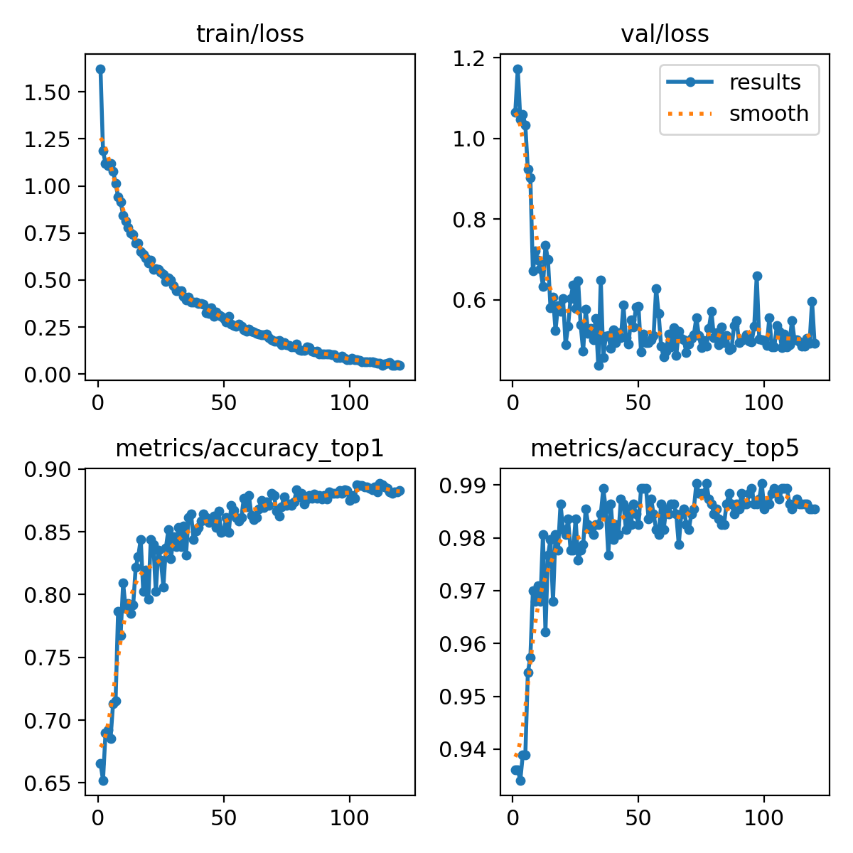
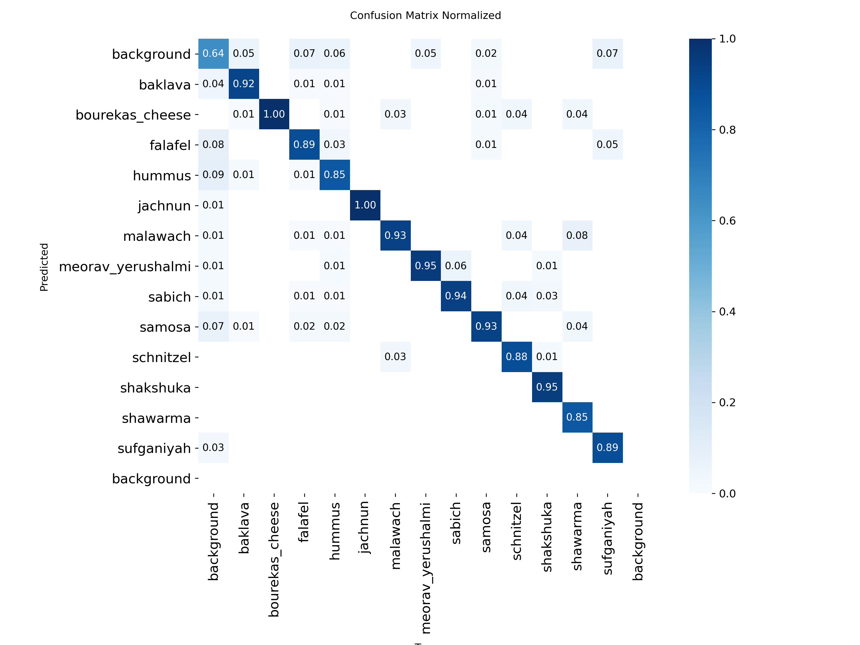
Reading the train-loss vs val-loss graph (what it actually means)
These two curves are the single most important diagnostic in training, and they tell a precise story. Both are the cross-entropy loss (with label smoothing): a number that is small when the model puts high probability on the correct class and large when it is wrong or unsure. They are computed on two different sets of images, and the comparison between them is what matters.
- Train loss (top-left) is measured on the images the model is actively learning from. It falls steadily from about 1.6 toward nearly 0. That only says the model is successfully memorising and fitting its training data, it says nothing on its own about whether it learned anything useful.
- Validation loss (top-right) is measured on held-out images the model never trains on. It is the honest signal of generalisation. Here it drops sharply for the first ~20 epochs, then plateaus around 0.5 and stays flat for the remaining 100 epochs.
- Healthy (what we have): val loss falls, then flattens. The model keeps getting better on train without getting worse on unseen data. The flat val loss plus still-rising val accuracy (bottom-left, to ~0.89) means the extra epochs are harmless.
- Harmful overfitting (what we do NOT have): val loss would bottom out and then turn back upward while train loss keeps falling. That U-shape is the signal to stop earlier. Our val loss never turns up, so the model is not overfitting in the damaging sense.
This is exactly why we do not deploy the last epoch: best.pt is saved at the epoch with the
highest validation top-1 (epoch 112), not the lowest train loss. Selecting on the held-out metric,
not the training metric, is what guarantees the shipped model is the best generaliser, and the
patience=25 early-stopping rule exists to cut the run if val ever did start to degrade. The
jagged look of the val curves is ordinary epoch-to-epoch noise on a finite validation set, not instability;
the dotted "smooth" line is just a moving average to make the trend readable.
What the confusion matrix shows
Each cell is the fraction of images of a true class (column) that the model predicted as a given class
(row); a perfect model is a pure diagonal. V2's diagonal is strong across all 13 real dishes (0.85 to
1.00: bourekas and jachnun at 1.00, sabich 0.94, malawach 0.93). The one deliberately weaker cell is
background at 0.64: it is a broad catch-all of many non-Israeli foods, so it is the hardest class,
and about a third of background images are still read as a look-alike dish (creamy foods leak toward
hummus, fried toward samosa/falafel). That residual is acceptable because the arbiter does not need
background to be the top-1 guess, it uses the probability i_p_background, which is
high on those foods even when another class edges it out, and that is enough to route them to the global
expert.
System Limitations and Future Work (V2 Architecture)
Limitation 1 · Classification backbone is not Pareto-optimal
The Global and Israeli experts use YOLO11l-cls. In its classification variant this is a
legitimate classifier (the detection head is removed), but the C3k2 backbone is co-designed for
multi-scale detection feature reuse, which is not the accuracy-per-FLOP optimum for single-label
classification. On ImageNet-1k, hierarchical and isotropic classifiers occupy a stronger frontier.
| Backbone | Params | IN-1k top-1 | Note |
|---|---|---|---|
| YOLO11l-cls (current) | ~13M | good | single exportable training and inference stack |
| Swin-T (Liu et al., ICCV 2021) | ~28M | 81.3% | shifted-window attention, hierarchical |
| ConvNeXt-T (Liu et al., CVPR 2022) | ~28M | 82.1% | modernized ConvNet, strong inductive bias |
Limitation 2 · The arbiter is information-starved (logits-only features)
The current arbiter consumes only scalar summaries of each expert's softmax: confidence, entropy, and margin. These are a deterministic, lossy function of the penultimate 1280-D embedding. By the data processing inequality, the embedding carries at least as much label-relevant information as any function of it:
I(domain ; conf, entropy, margin) ≤ I(domain ; embedding_1280)
The information we discard is exactly the visual-feature overlap that defeats margin-based routing (falafel vs crab_cakes, sabich vs global dishes). A multimodal arbiter on the concatenated penultimate embeddings of both experts routes on visual evidence, not probability shape alone.
Limitation 3 · No native Open Set Recognition for out-of-domain inputs
The Israeli expert is overconfident on food it never saw, and we delegated the entire correction to the downstream arbiter. This treats the symptom. The Open Set Recognition literature provides root-cause fixes that force low confidence on non-Israeli inputs natively:
| Method | Mechanism | Reference |
|---|---|---|
| Background / "unknown" class | Add a class of global foods so the softmax has a sink for OOD | standard practice |
| Outlier Exposure | Train against an auxiliary OOD set to flatten OOD confidence | Hendrycks et al., ICLR 2019 |
| Energy-based OOD | Score by free energy of logits; cleaner separation than softmax | Liu et al., NeurIPS 2020 |
| OpenMax | Recalibrate logits with extreme-value theory to expose unknowns | Bendale & Boult, CVPR 2016 |
| MSP baseline | Maximum softmax probability as an OOD score | Hendrycks & Gimpel, ICLR 2017 |
A real attempt: fine-tuning on tagged demo images (and why it failed)
The data-tagging flywheel in the live demo produces labelled real-world captures, so the obvious next
step is to fine-tune the Israeli expert on them. We tried it four times on the worst real-world
class, hummus, with a safety harness that never touches the production weights, holds out
part of the tagged set, and re-validates on the original clean test split. Every run made the model
worse, and the regression guard correctly refused to recommend all four.
| Run | Setup | Clean test top-1 (was 92.26%) | Change |
|---|---|---|---|
| 1 | 15 epochs, AdamW, lr 1e-4, full fine-tune, 21 tagged images ×8 aug | 49.89% | −42.4 pts |
| 2 | 25 epochs, froze the backbone and trained the classifier head only | 23.37% | −68.9 pts (collapsed: the framework reset the head to random and a frozen backbone could not retrain it) |
| 3 | 20 epochs, lr 1e-4, 72 tagged ×2 aug | 66.21% | −26.1 pts (least bad) |
| 4 | 15 epochs, lower lr 5e-5, 72 tagged ×1 aug | 52.64% | −39.6 pts |
What would actually fix it
| Fix | Why it addresses the failure |
|---|---|
| Rehearsal / replay | Mix the original balanced training data back in (not just the new class) so shared features are not overwritten. Naive fine-tuning on one class guarantees forgetting. |
| Freeze the backbone, retrain the head WITHOUT resetting it (or LoRA) | The "head" is the small final classifier layer; the "backbone" is the feature extractor. Runs 1, 3, 4 fine-tuned every layer; run 2 froze the backbone but the framework reset the head to random, so it could not recover. The correct version keeps the existing head weights (or adds low-rank adapters), adapting only the classifier while leaving the learned features intact, with far less data. |
| Hard negatives for the look-alike neighbours | Since the new hummus images resemble their neighbours, add labelled examples of those neighbours (or a contrastive / triplet objective) so the boundary is sharpened instead of swallowed. |
| Curate, do not just collect | Drop ambiguous borderline captures; keep class-balanced sampling so the new images do not dominate. A heavy augmentation multiplier on a tiny, ambiguous set (run 1, ×8) makes the overfitting worse. |
| Early-stop on the clean-test metric | Select the checkpoint by overall held-out accuracy, not by the new class's accuracy, so a gain on one class can never be bought with a loss everywhere else. |
| Fix the root cause at the data level | The binding constraint is training viewpoint, not one class. The durable answer is multi-viewpoint (including top-down) data for all classes plus a stronger backbone, not patching a single class after the fact. |
V2 synthesis: which lever moves which number
| V2 change | Error pool attacked | Effect on realized acc | Effect on oracle |
|---|---|---|---|
| ConvNeXt-T / Swin-T backbone | both-experts-wrong (11.34%) | up | raises it |
| Embeddings arbiter (2560-D) | routing error (4.91%) | up, toward oracle | unchanged |
| OSR on the Israeli expert | routing error + Israeli recall | up, toward oracle | unchanged |
System Analysis V2 (after the open-set retrain)
This is the full system evaluation after the Israeli Model V2 retrain (the open-set
background class plus the i_p_background arbiter feature). The original
System Analysis tab is kept unchanged as the V1 baseline; this tab is the current production system,
measured on the held-out test set of 11,352 images (regenerated
datasets/system_evaluation.csv).
Error decomposition (V2)
Every outcome on the test set, split into the three mutually exclusive buckets that tell you where the remaining errors live.
- Routing error 2.7% (301 images): a correct expert existed but the arbiter sent the image to the other one. This is the only bucket a better arbiter can recover, and V2 already cut it from the V1 4.9% down to 2.7% (the open-set signal). It is now a small pool.
- Both models wrong 11.2% (1,270 images): neither expert was right, so no router could have helped. This is the real ceiling, and it only moves with better models or more data (a stronger backbone), not with routing. It defines the 88.8% oracle.
- The takeaway: the arbiter side is nearly solved (2.7% recoverable left); the remaining headroom is in the experts, exactly as the Limitations and V2 tab argues.
Accuracy by domain (V2)
| Slice | Images | System | Always-global | Oracle |
|---|---|---|---|---|
| Global domain | 9,960 | 87.3% | 88.2% | 88.2% |
| Israeli domain | 1,392 | 77.9% | 0.0% | 93.2% |
| Overall system | 11,352 | 86.2% | 77.4% | 88.8% |
V1 vs V2, side by side
| Metric (held-out test) | V1 | V2 | Change |
|---|---|---|---|
| System top-1 | 83.8% | 86.2% | +2.4 |
| Israeli-domain accuracy | 60.8% | 77.9% | +17.1 |
| Routing ROC-AUC | 0.933 | 0.973 | +0.040 |
| Routing error pool | 4.9% | 2.7% | -2.2 |
| Both-wrong pool | 11.3% | 11.2% | ~same (model-bound) |
Top remaining system confusions (V2)
The misses left after V2, true class to predicted class on the test set. They are dominated by genuine visual look-alikes, which is the both-models-wrong pool, not routing.
| True | Predicted | Count | Note |
|---|---|---|---|
| falafel | crab_cakes | 35 | brown fried balls, the classic confuser |
| chocolate_mousse | chocolate_cake | 12 | same ingredient family |
| apple_pie | bread_pudding | 10 | baked, similar texture |
| falafel | tacos | 10 | both global; model error, not routing |
| hummus | omelette | 10 | pale, creamy, similar plating |
| samosa | spring_rolls | 9 | fried dough pockets |
Approaches We Tried and Rejected
Before settling on a BLE gravimetric scale for weight, we built and measured two other ways to get the mass of the food. Both worked in the lab and both were rejected for concrete, measured reasons. Keeping this record is the honest engineering story, and it is the direct answer to "why a scale and not just the camera?"
Approach A · Estimating weight from a single photo (volume to mass)
The idea: put a coin of known size in frame as a fiducial (an Israeli 1 shekel coin, 18 mm), use it to convert pixels to centimetres, recover the food's volume, then multiply by density to get grams. We implemented two independent volume methods and validated both against a gold standard.
Method 1 · Monocular depth (MiDaS)
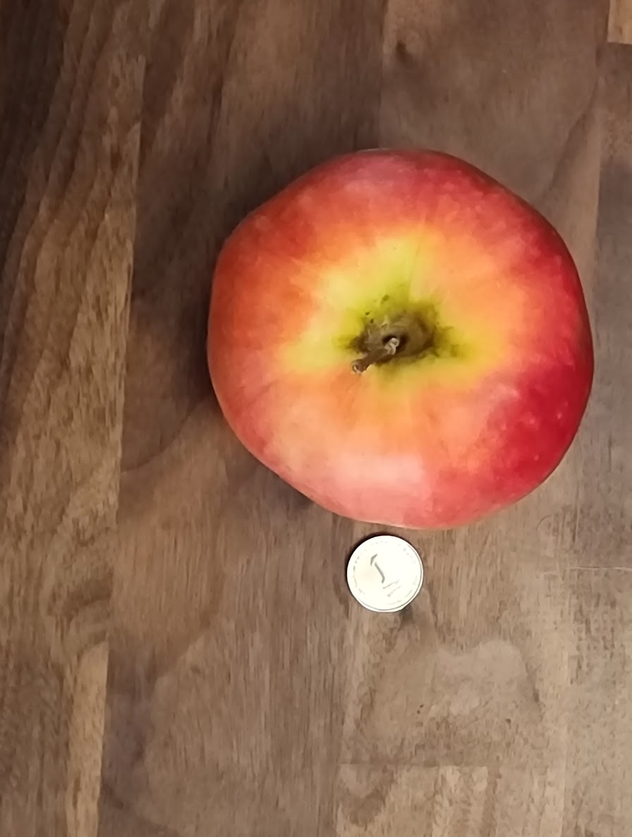
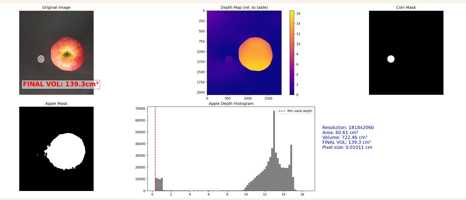
A neural depth network estimates the height of every pixel above the table; summing height over the food's area gives a volume. It got the apple to 139.3 cm³.
Method 2 · Shadow geometry
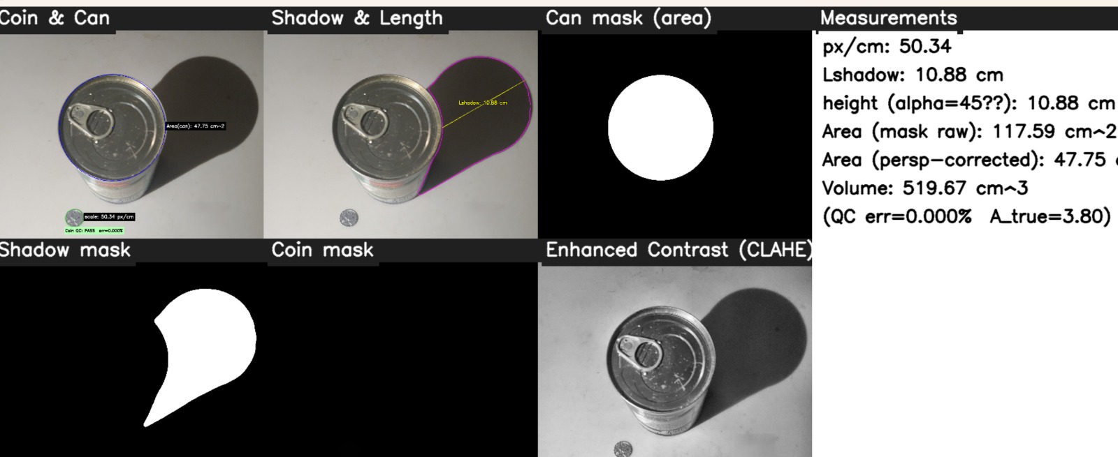
With a 45° light, an object's height equals the length of its cast shadow. Multiplying the perspective-corrected top area by that height gives a volume without any depth network, purely geometry.
Validation: Archimedes water displacement (the gold standard)
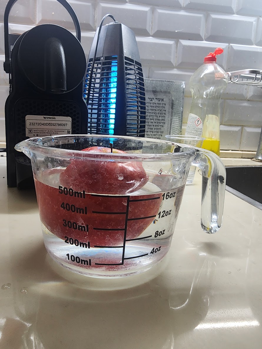
- Volume is not mass. Converting cm³ to grams needs density, and density varies wildly by food (a cup of salad versus a cup of peanut butter). At inference the density is unknown, so even a perfect volume gives a wrong weight. This is the fatal flaw.
- It only worked in controlled conditions. It required a coin in frame, a single clean object, a plain background, and (for the shadow method) a hard directional light. A real plate of mixed food breaks all of these.
- Errors compound. Fiducial detection, segmentation, depth or shadow estimate, then a density guess, each multiplies the next. The apple floated and had to be forced under for even the validation.
Approach B · Reading the kitchen scale's display by OCR
The next idea kept a real scale but avoided pairing it electronically: point the camera at the scale's
7-segment LCD and read the number with OCR (pytesseract, in
food_app.py / new_gui_with_ocr.py).
The decision: read mass at the source over BLE
Both rejected routes share one mistake: inferring a physical quantity the hardware already measures exactly. The scale computes grams internally, so instead of photographing its screen we reverse-engineered its Bluetooth Low Energy protocol and read the mass directly (see the BLE Scale tab). No density assumption, no fiducial, no lighting or glare dependence, gram-accurate every time.
| Approach | Lab result | Why rejected |
|---|---|---|
| MiDaS depth volume | apple 139.3 cm³ (~7% vs Archimedes) | volume needs density to become grams; controlled-conditions only |
| Shadow geometry volume | can 519.67 cm³ | same density problem; needs a coin and a hard shadow |
| 7-segment OCR of the scale | worked on clean frames | glare, angle, flicker, segmented-font OCR is unreliable |
| BLE gravimetric (chosen) | exact grams at the source | robust, no inference, no assumptions |
Training Lab: how learning actually happens
Three interactive toys that make the training terms concrete: how a model learns by gradient descent (and why the learning rate matters), why batch size changes the path, and what a backbone, a head, and freezing really mean. These are the exact levers behind the Israeli Model V2 retrain and the fine-tune failures.
1 · Gradient descent and the learning rate
A model "learns" by minimising a loss (how wrong it is). It repeatedly nudges its weights downhill along the slope (the gradient) of the loss. The step size is the learning rate (LR). The curve below is a simple loss bowl; the dot is the current weight. Press play and change the LR.
| LR regime | What you see | Why |
|---|---|---|
| Too small (≈0.1) | The dot crawls, barely moves | Tiny steps; training would take forever / stall |
| Good (≈1.0) | Slides smoothly to the bottom | Steps are proportional to the slope; fast, stable convergence |
| High (≈1.9) | Overshoots and zig-zags, still settles | Each step jumps past the minimum but the bowl pulls it back |
| Too high (>2.0) | Bounces outward and diverges | Steps overshoot more than the slope corrects; loss explodes (this is what too-high LR does in real training) |
lr0=0.001 in our training is small on purpose: it adapts the model without
blowing up the pretrained features. warmup ramps the LR up gently at the start for the same reason.2 · Batch size: why it changes the path
The true downhill direction is computed by averaging over data. A batch is how many images you average before each step. A small batch gives a noisy estimate of the slope (the path jitters); a large batch gives a smooth estimate (a cleaner path) but each step costs more memory. Drag the batch size and watch the descent path on a 2-D loss (the rings are contours).
| Batch | Gradient | Trade-off |
|---|---|---|
| Small (1-8) | Noisy, jittery path | More updates per epoch, low memory, the noise can even help generalisation, but unstable BatchNorm statistics |
| Large (128+) | Smooth, direct path | Stable and fast on a GPU, but uses much more memory and can generalise slightly worse |
3 · Backbone, head, and freezing
A classifier has two parts. The backbone is the deep stack that turns an image into a compact feature vector (it holds the general visual knowledge). The head is the small final layer that maps that vector to class scores. Learning flows forward (prediction) then backward (the gradient updates the weights). Freezing the backbone locks it so only the head learns. Toggle freeze and run a step.
| Mode | What trains | When to use it |
|---|---|---|
| Full fine-tune (no freeze) | Backbone + head both update | Plenty of data; willing to risk catastrophic forgetting. Runs 1, 3, 4 of our fine-tune did this. |
| Freeze backbone, train head | Only the head updates; features stay intact | Little data; fast; protects general features. The right way to add a class cheaply. |
| Freeze backbone + reset head (the trap) | Head starts random, backbone cannot adapt to it | Never. This is exactly run 2 and the global fine-tune: the framework reset the head to random, the frozen backbone could not retrain it, and accuracy collapsed to near-random. |
4 · Logits, softmax, and what the arbiter reads
The final layer of each model outputs one raw score per class, the logits. They are unbounded
(any real number) and do not sum to anything. Softmax turns them into probabilities that
sum to 1, by exponentiating and normalising: p_i = e^(z_i/T) / Σ e^(z_j/T). The model's
"confidence" is just the largest probability. Drag the logits and watch the probabilities, and the three
numbers the arbiter actually consumes: top-1 confidence, margin, and entropy.
| Quantity | Meaning | Used by the arbiter as |
|---|---|---|
| logits (z) | raw, unbounded class scores, straight out of the final layer | not directly; they are turned into probabilities first |
| softmax probabilities (p) | logits squashed to [0,1], summing to 1 | g_conf1..5, i_conf1..5, and i_p_background |
| top-1 confidence | the largest probability (how sure the model is) | g_conf1, i_conf1, the gates |
| margin | top-1 minus top-2 (how decisive the choice is) | g_margin, i_margin |
| entropy | spread of the whole distribution (low = peaked, high = unsure) | g_entropy, i_entropy |
| temperature (T) | divides the logits before softmax: high T softens, low T sharpens | the calibration lever discussed in Limitations & V2 |
background class fixed.Real-World Image Validation
47 real photos of food taken with our own phones, sorted into class folders and run through the exact deployed pipeline offline. The folder name is the ground truth; none of these images were in training. Each tile is the evidence card the pipeline emits (the ROI it saw, both experts’ top-5, the arbiter’s decision). Click any card to enlarge.
Capture provenance - these are our own photos
Every original keeps its EXIF metadata, traceable to the device and moment of capture, 2016-11-12 to 2026-06-07. Most were shot on a Google Pixel 10 Pro in 2026, after the models were trained. Nothing was scraped from the web.
Accuracy by class
The 7 errors, by root cause
falafel
1/1 = 100%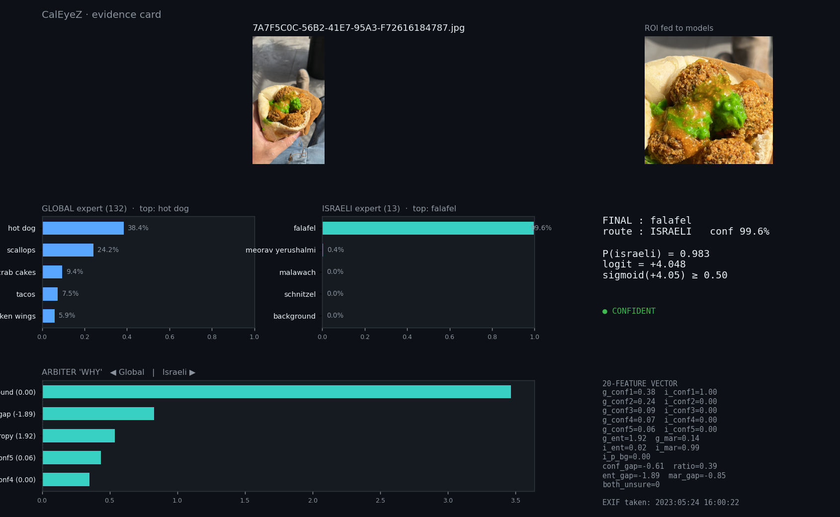
french fries
2/2 = 100%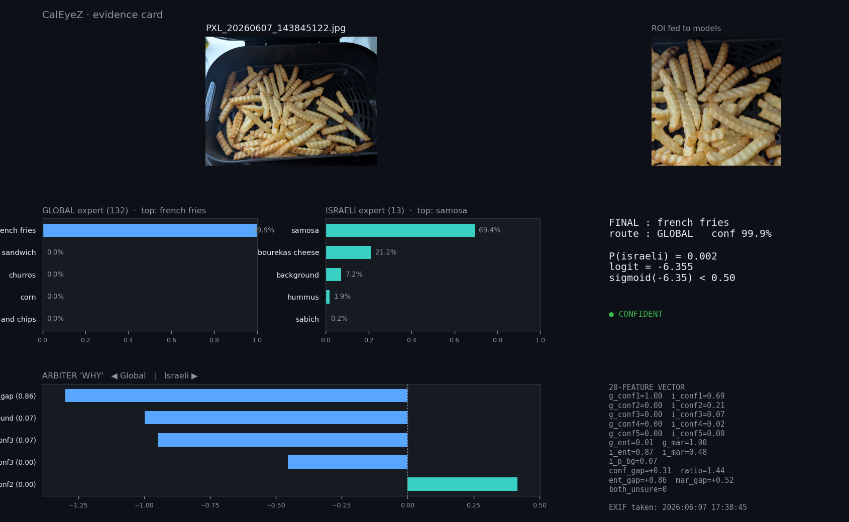
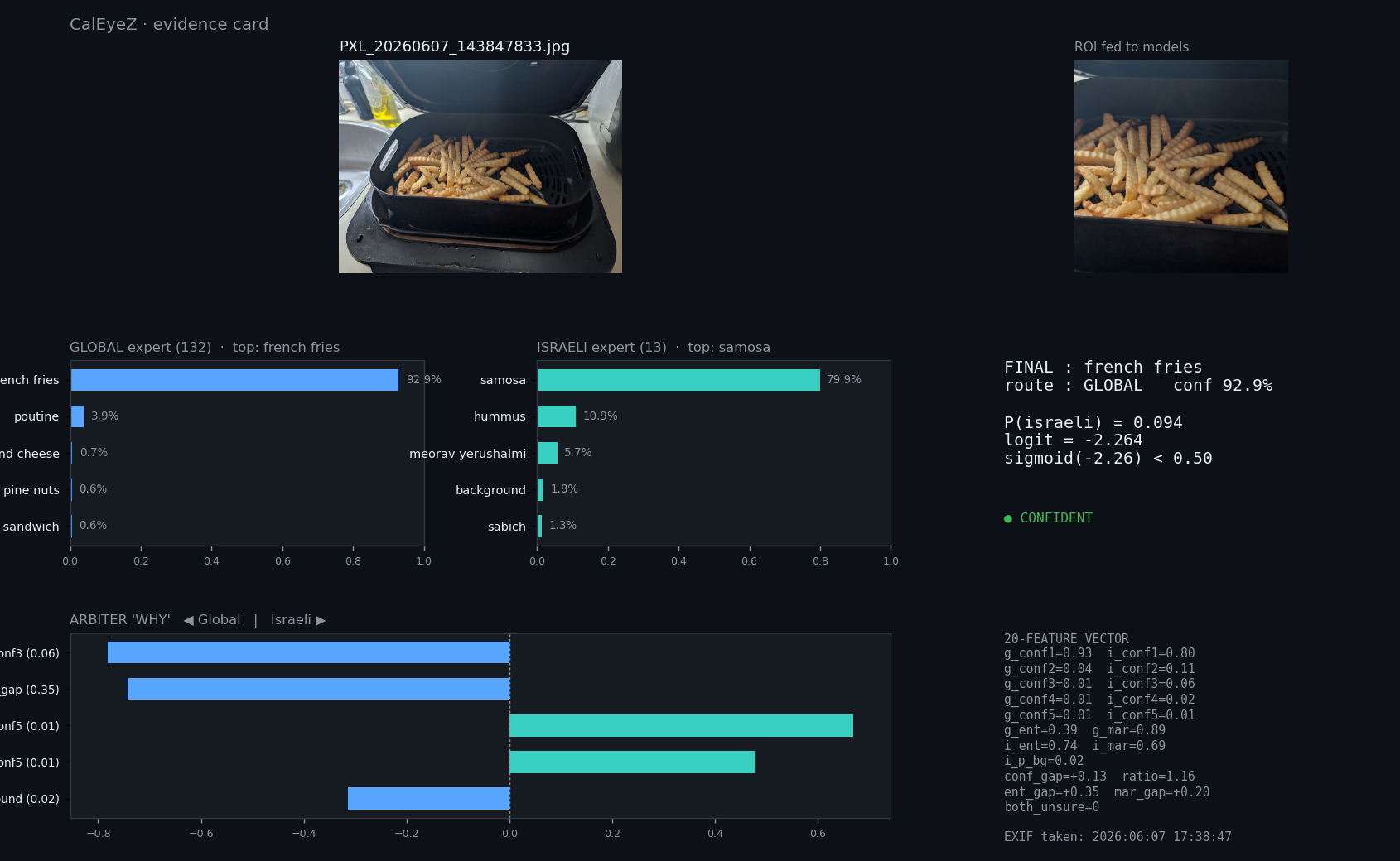
hamburger
12/12 = 100%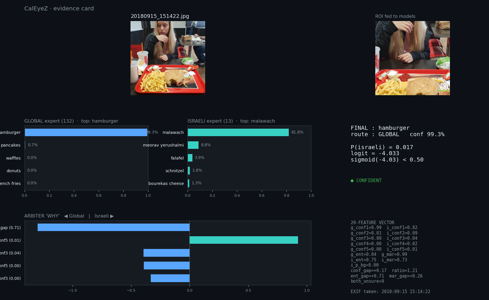
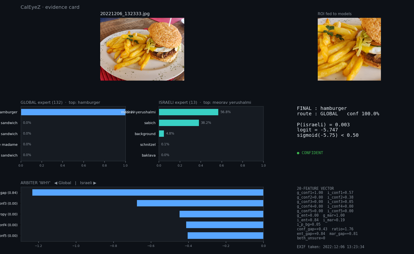
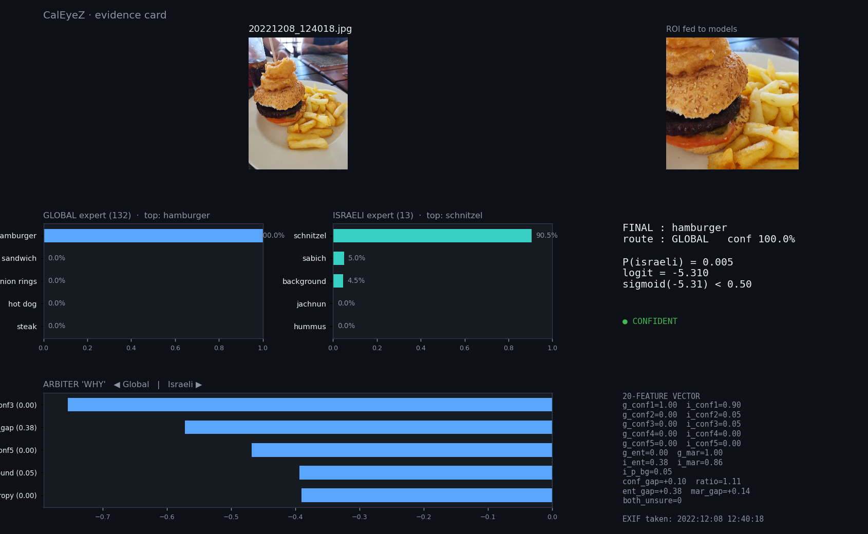
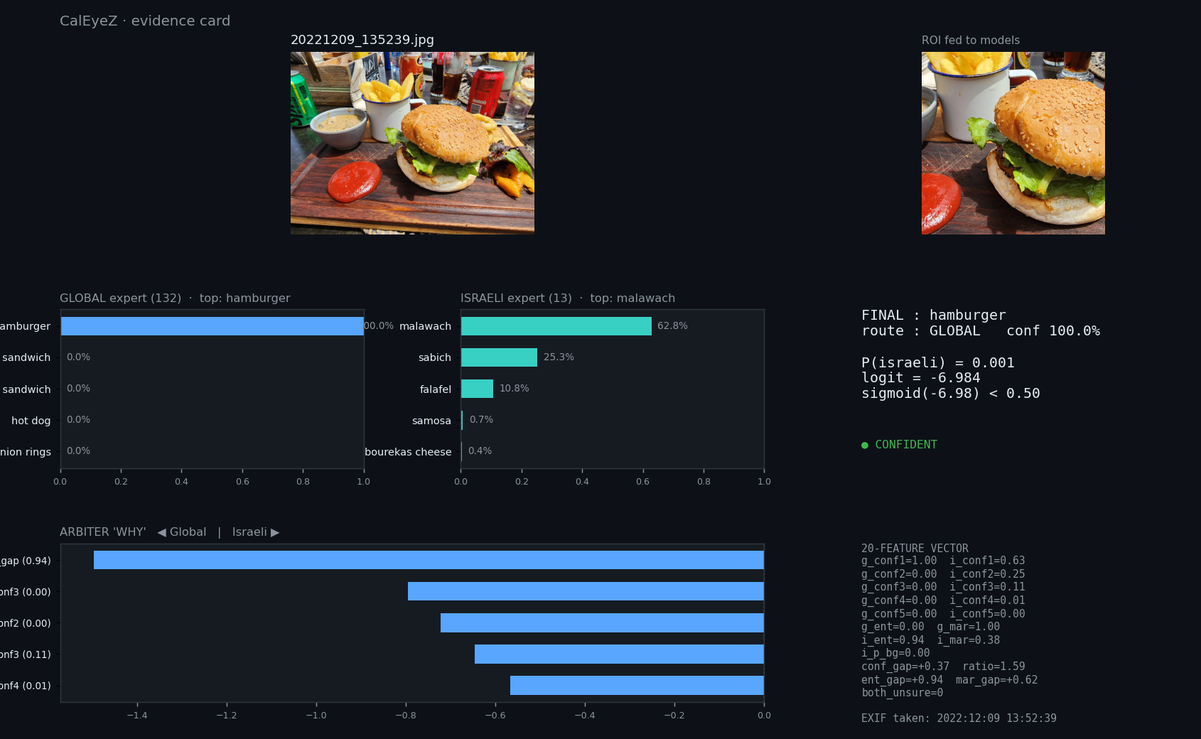
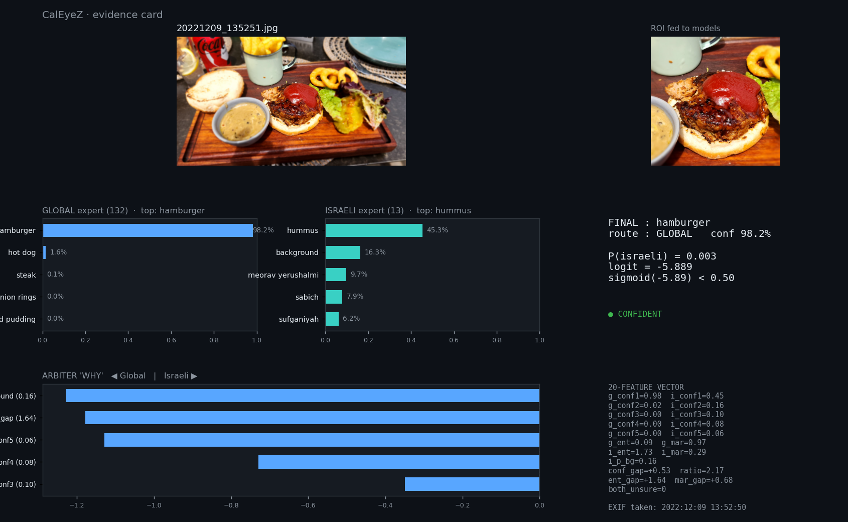
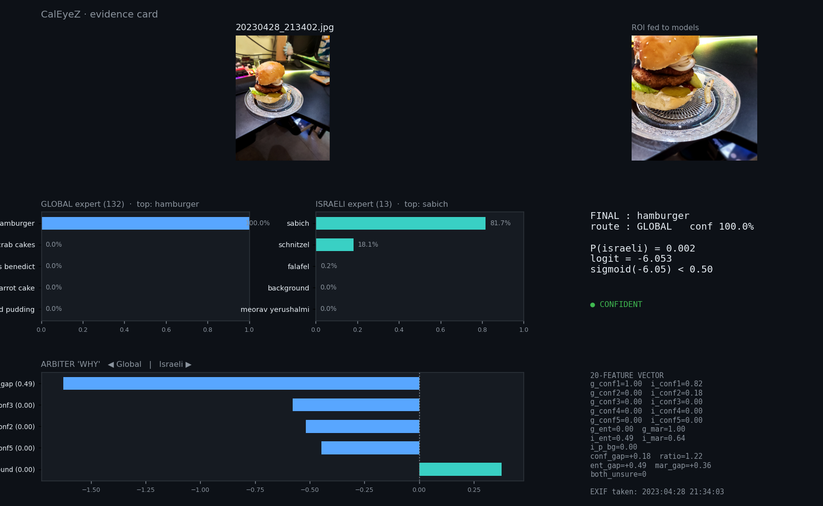
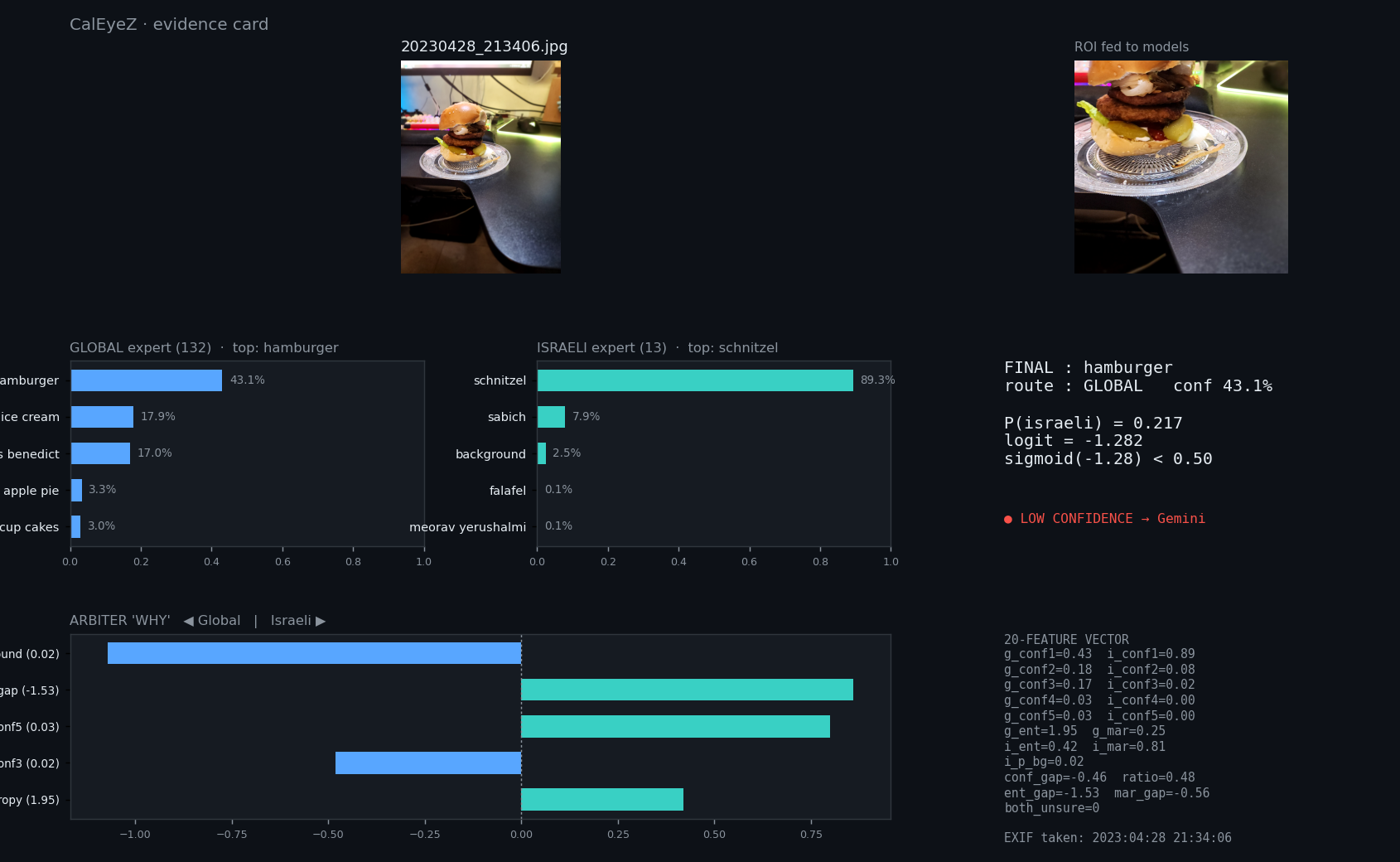
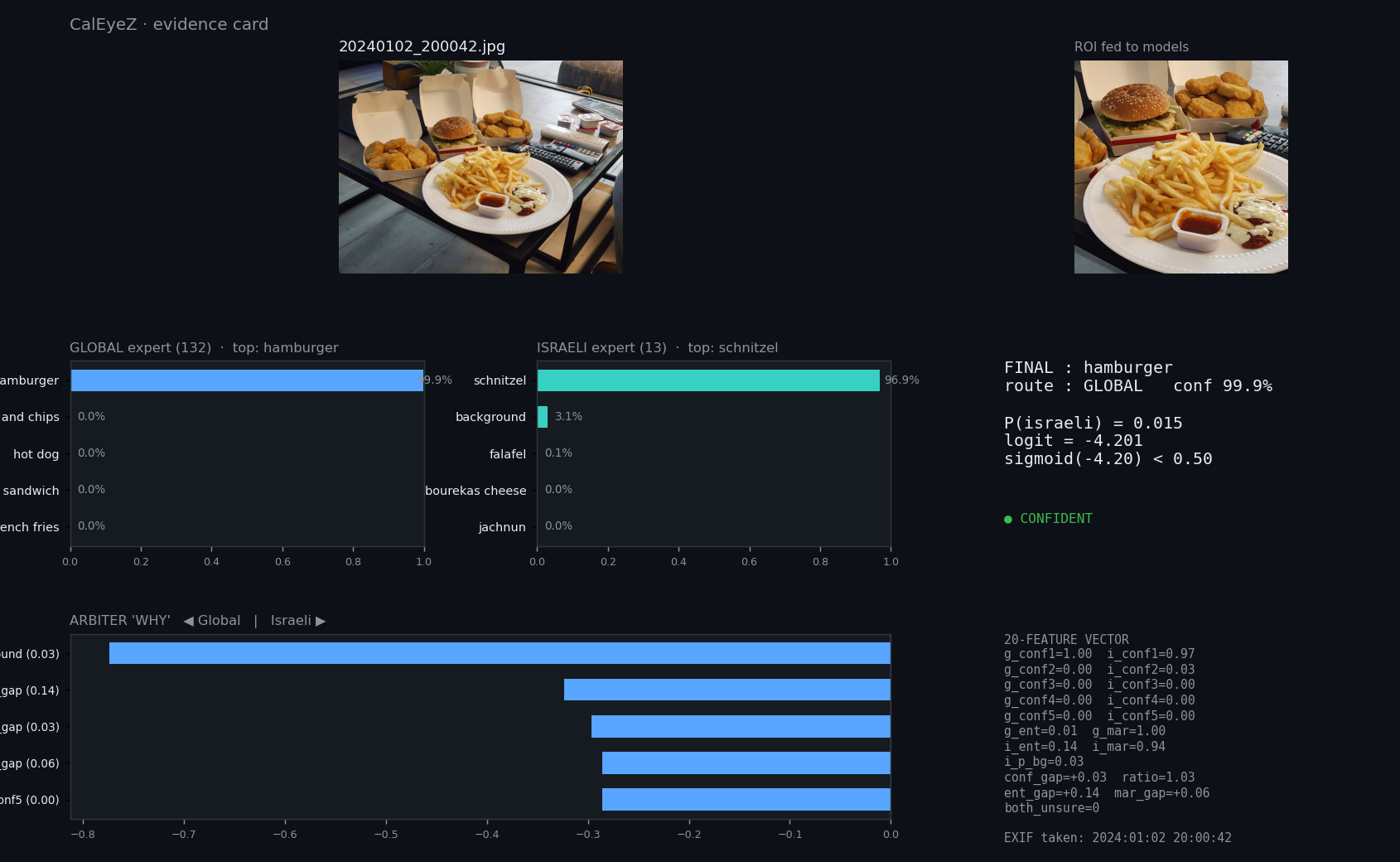
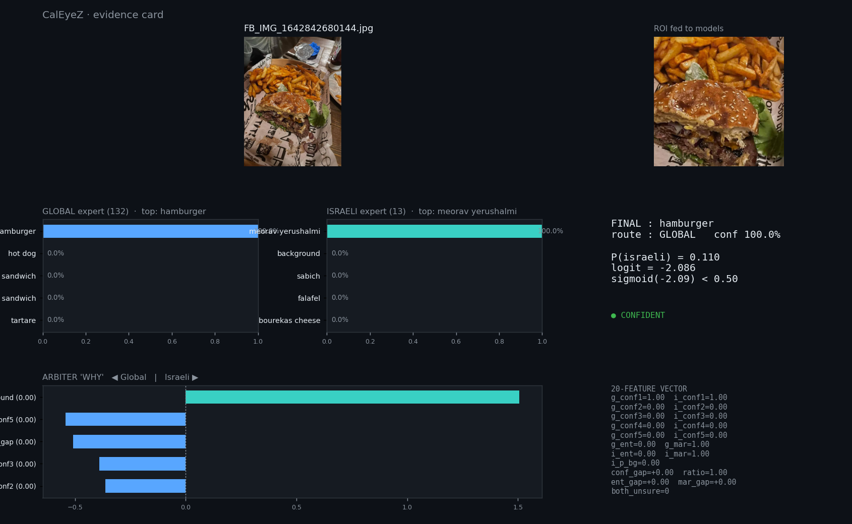
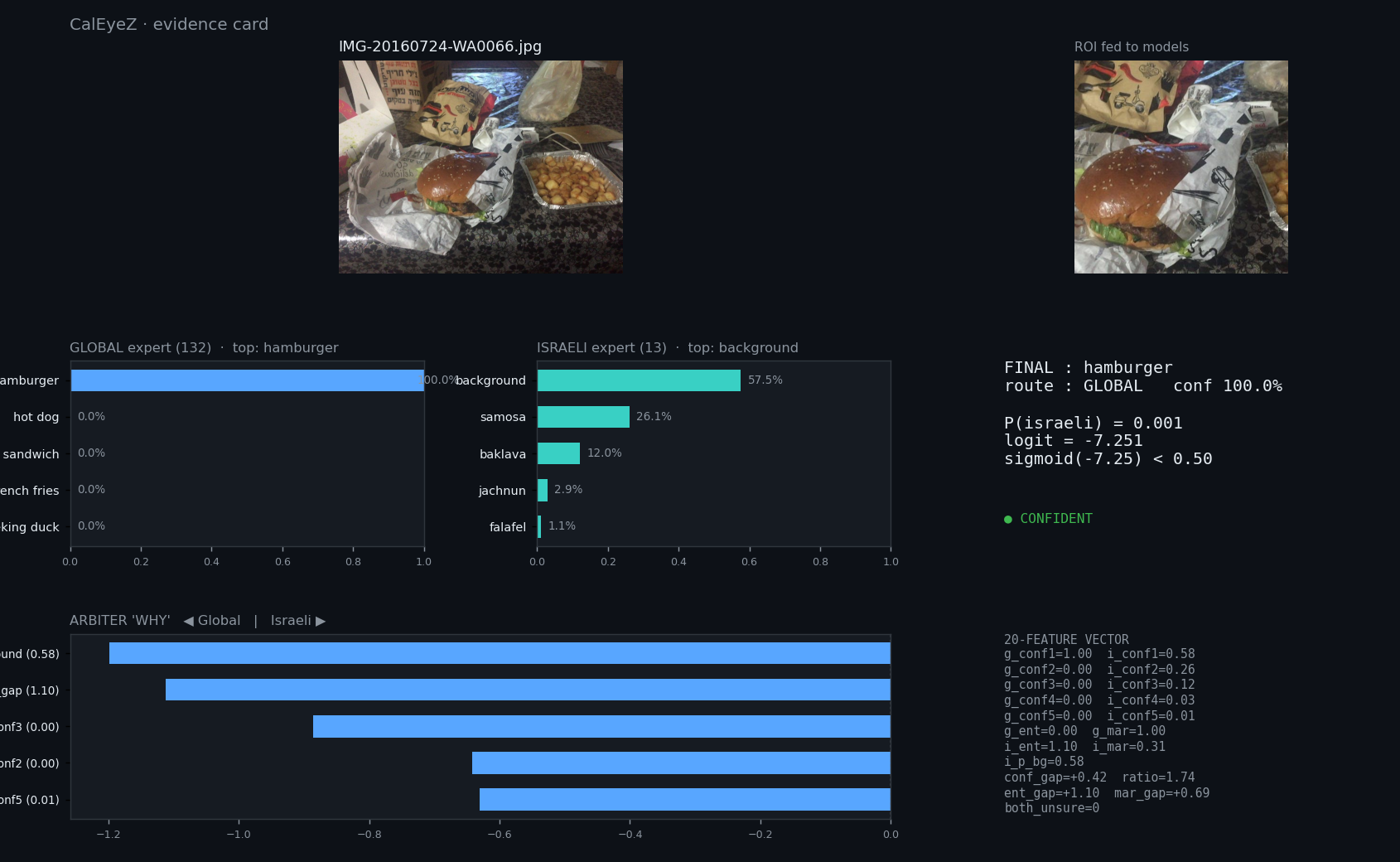
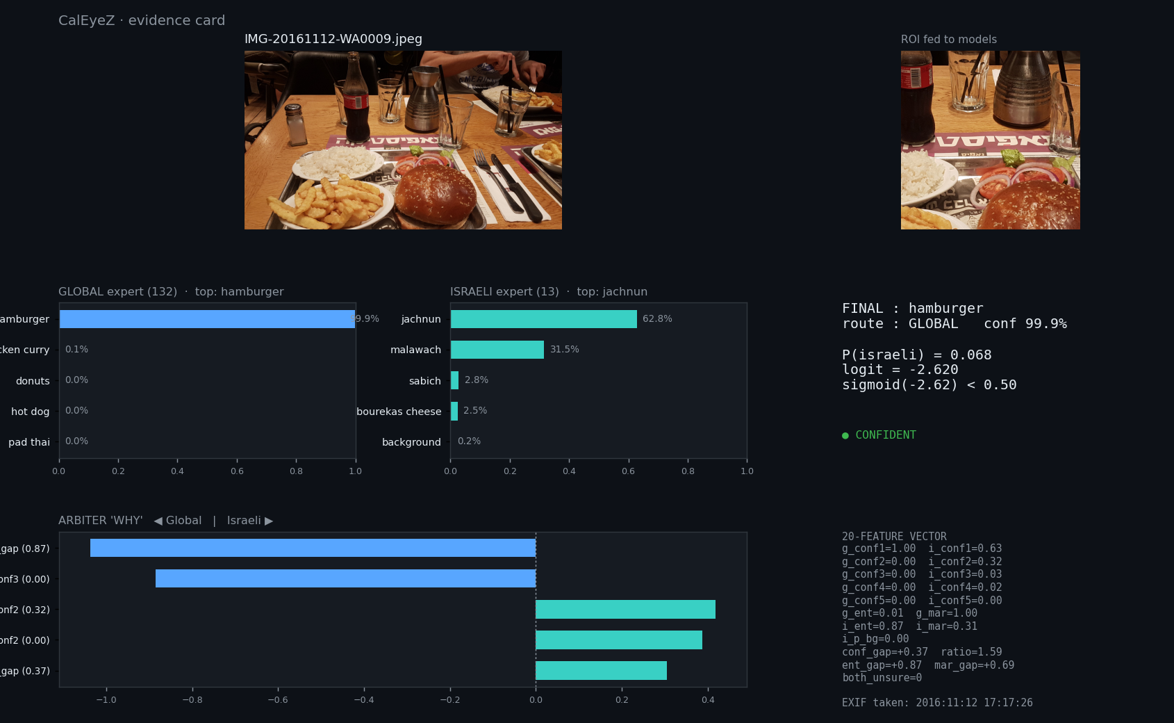
__card.png)
sabich
1/1 = 100%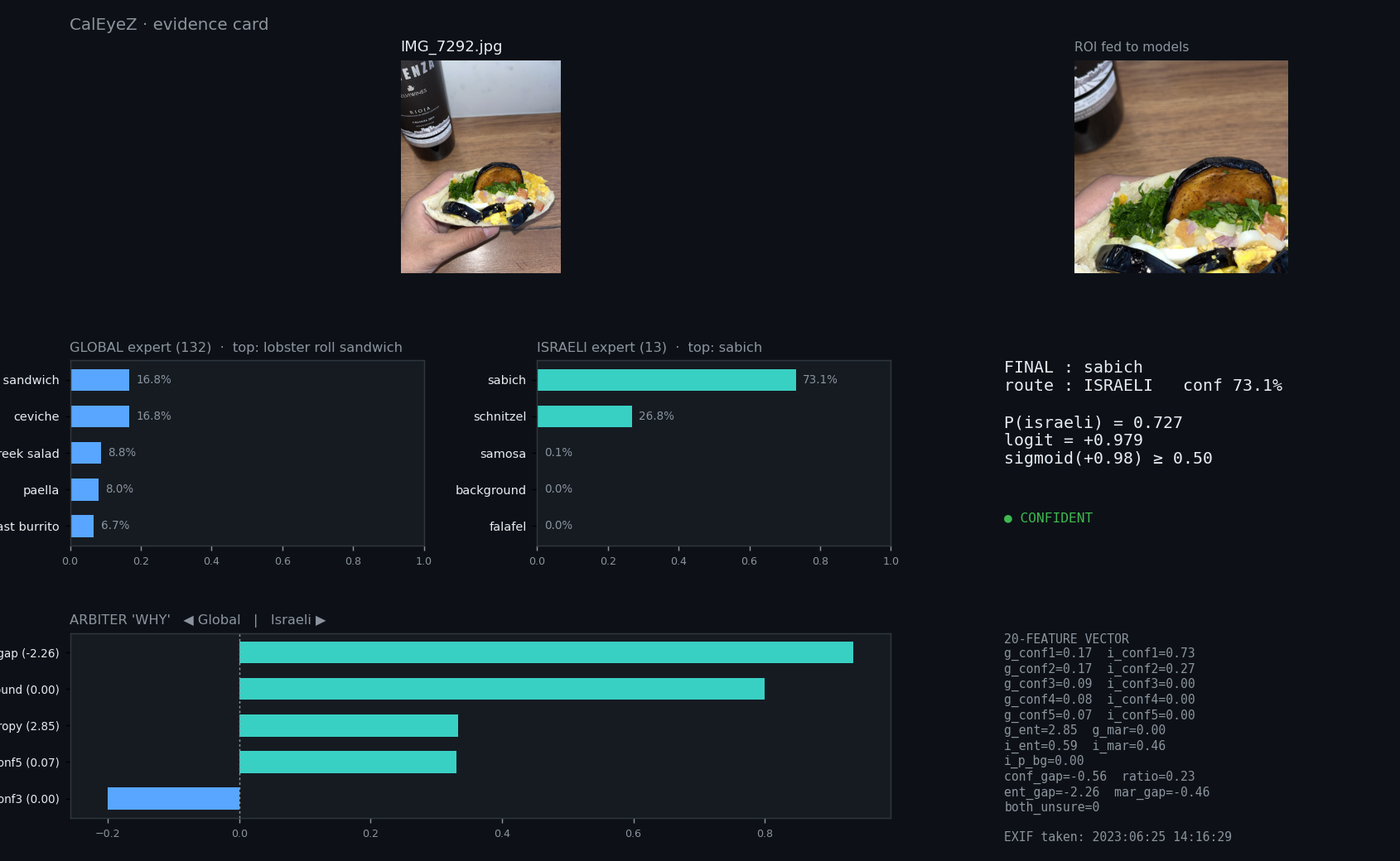
bourekas cheese
9/10 = 90%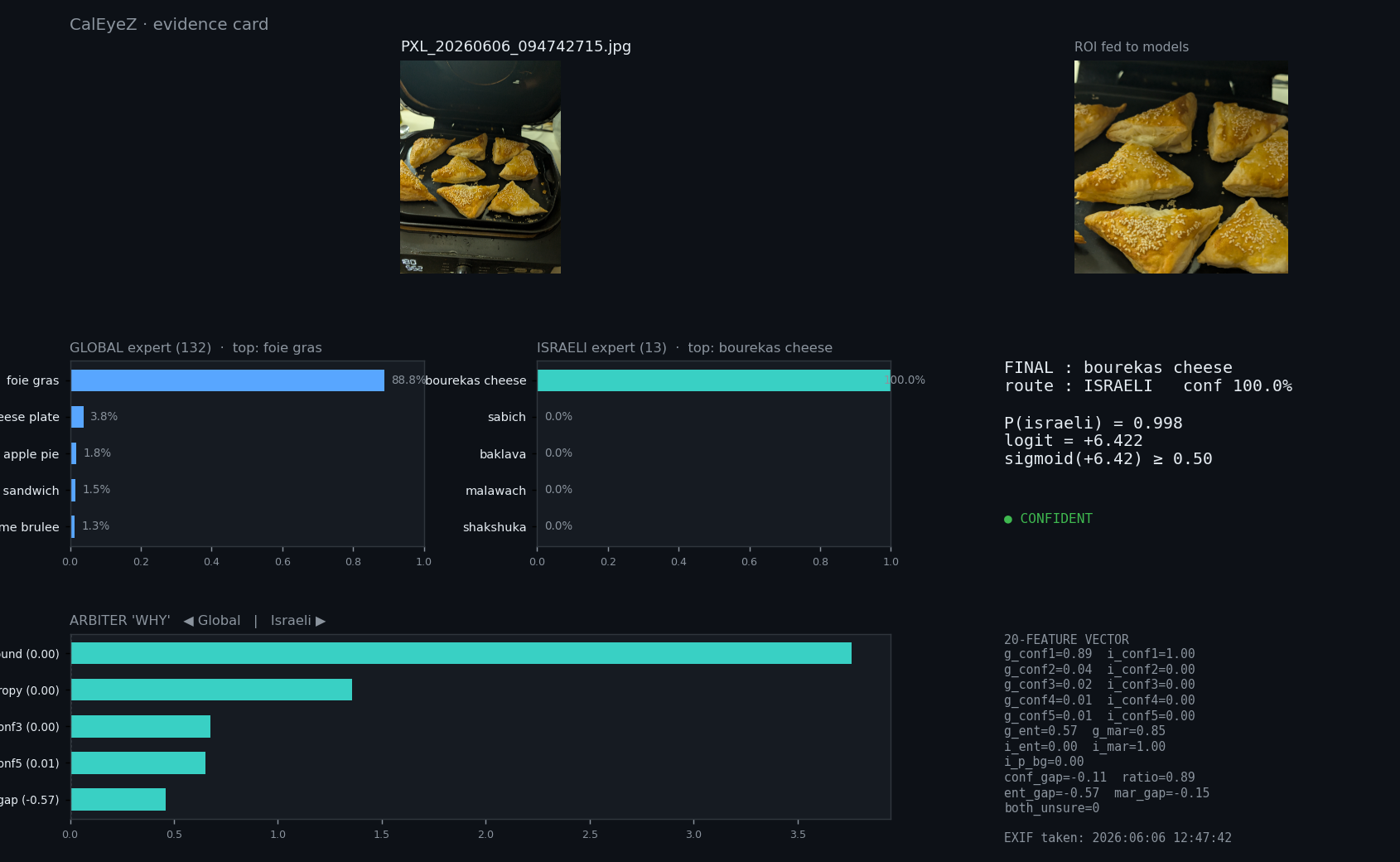
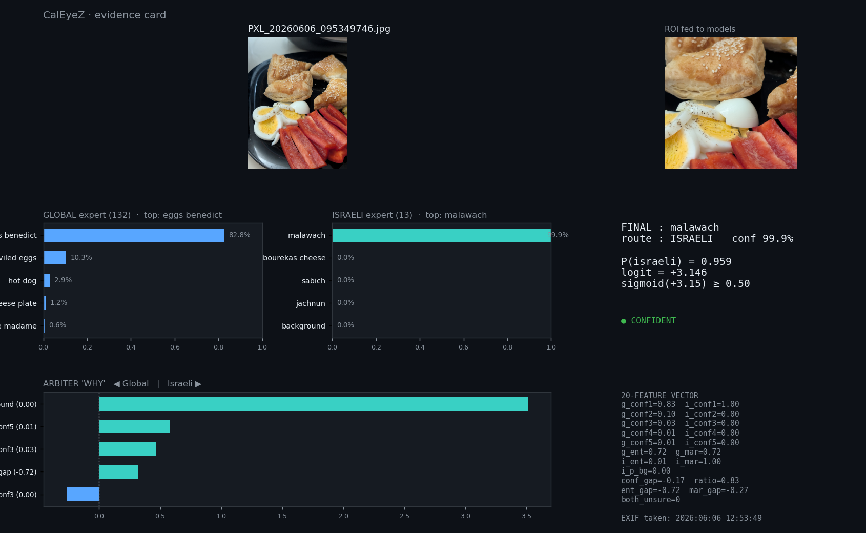
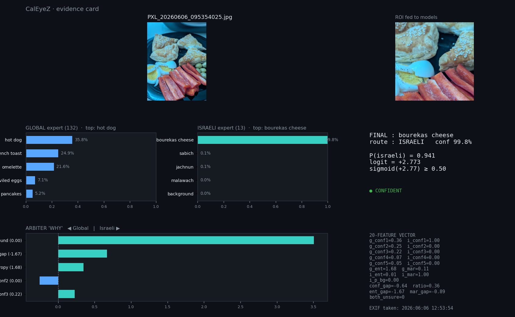
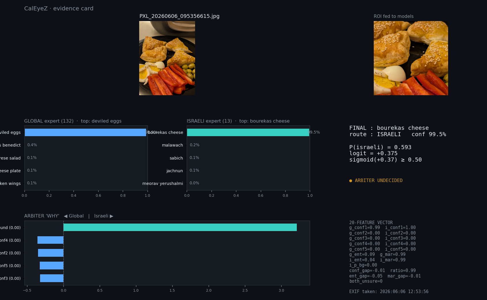
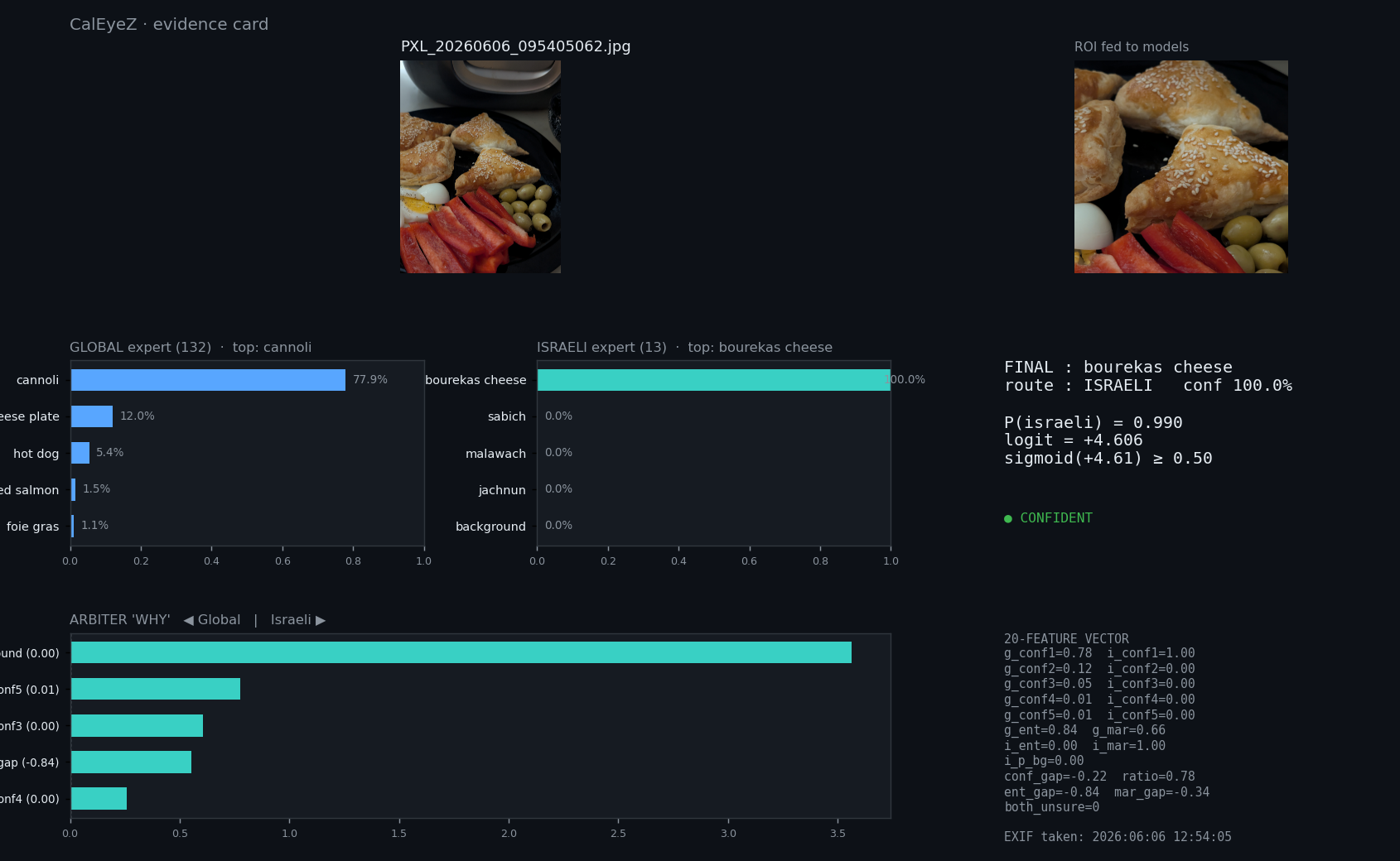
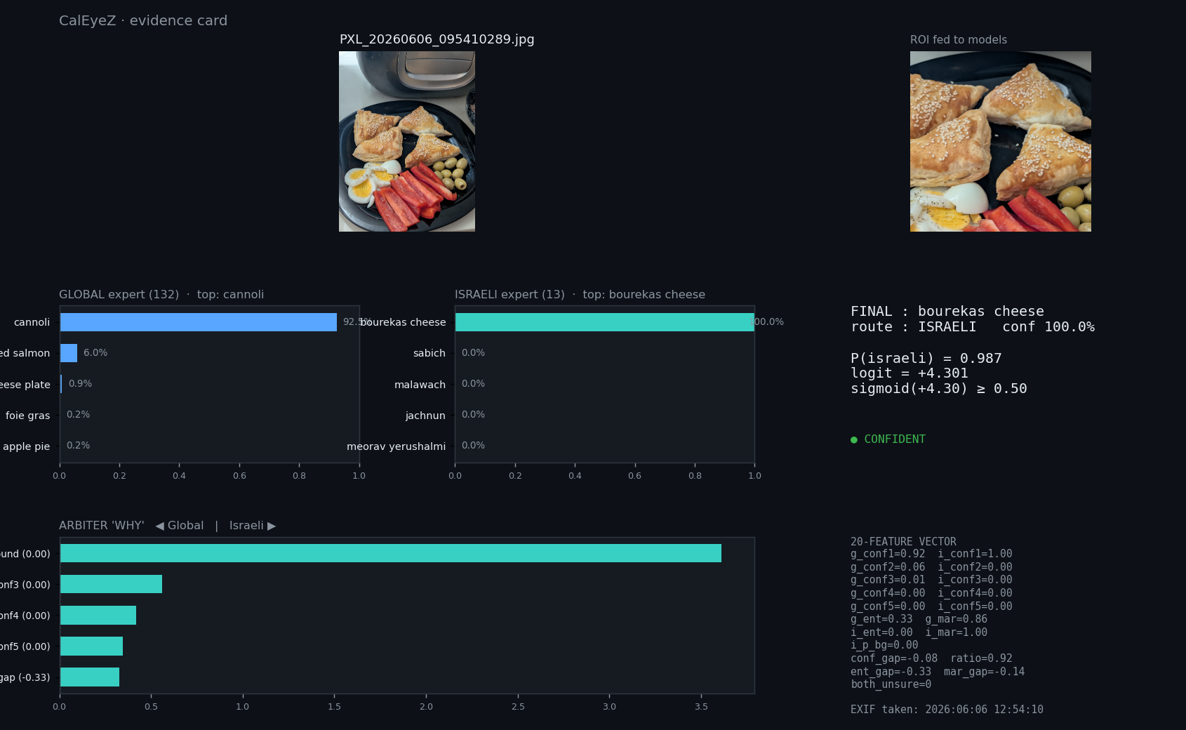
ice cream
3/4 = 75%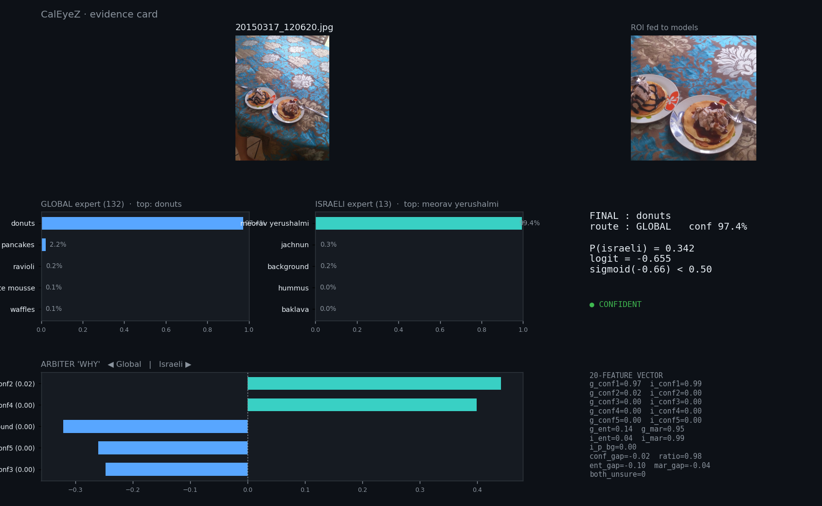
__card.png)
__card.png)
__card.png)
canned tuna
8/11 = 73%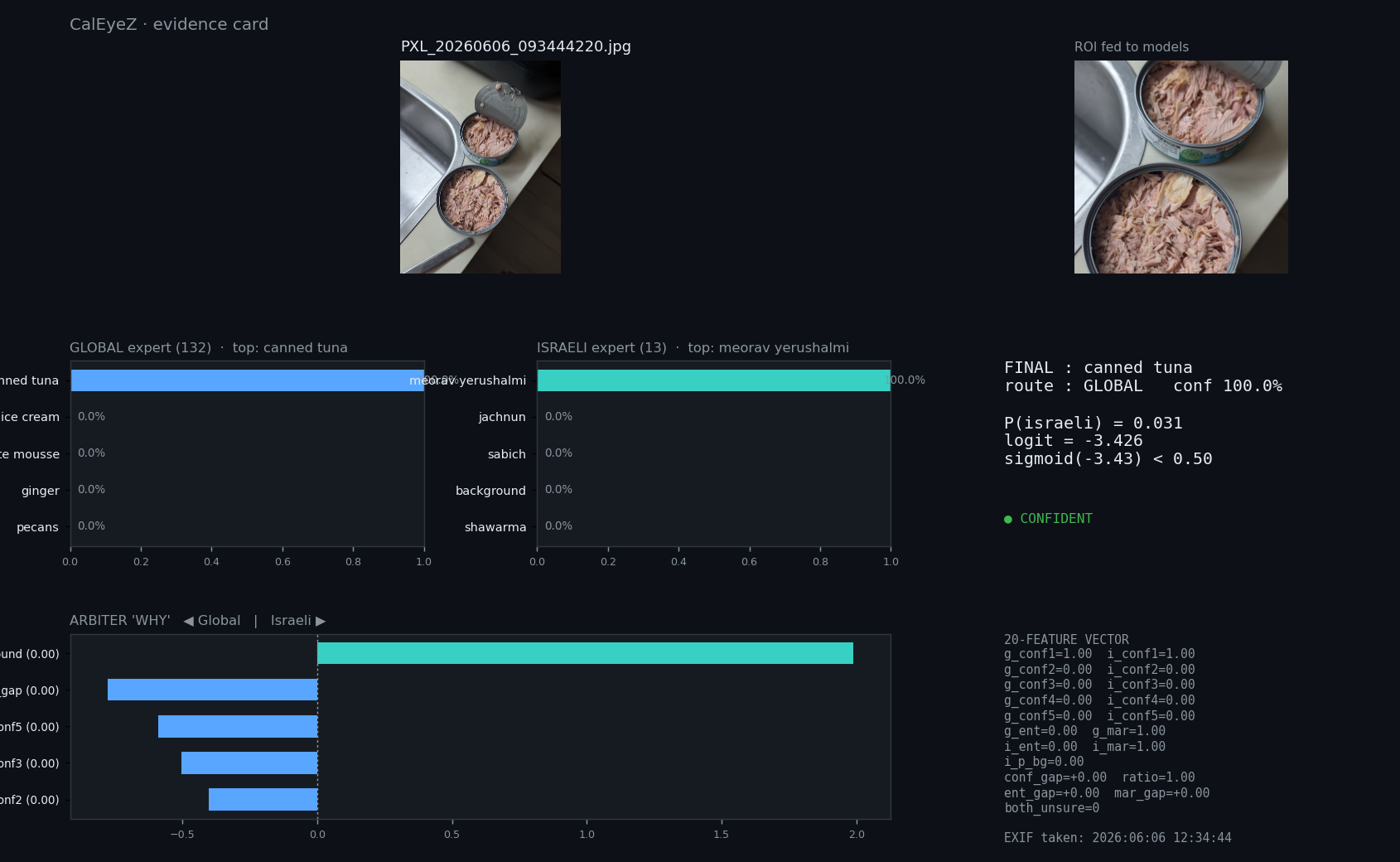
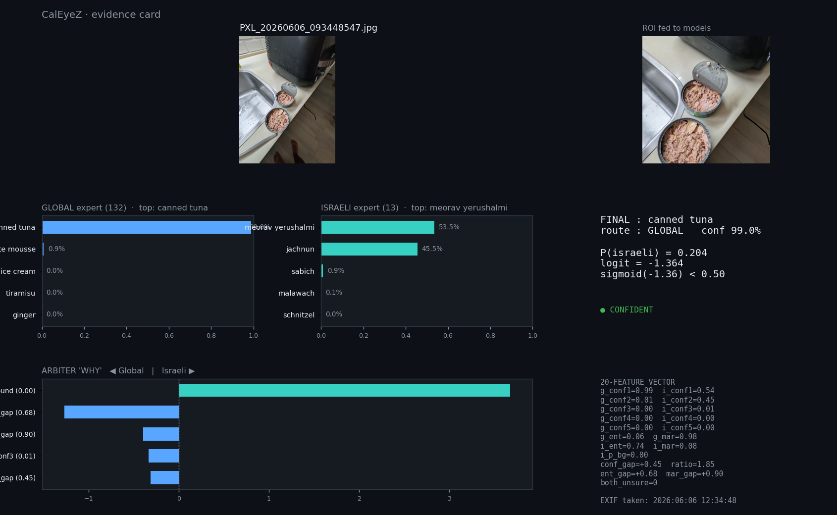
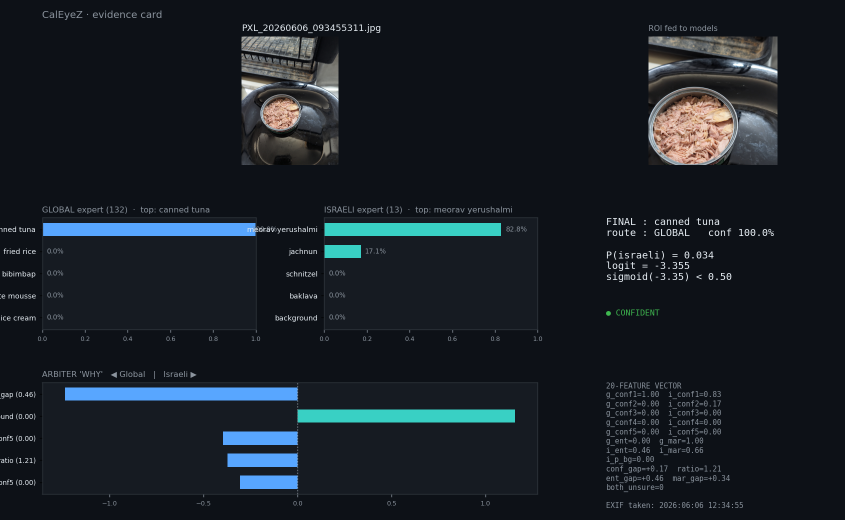
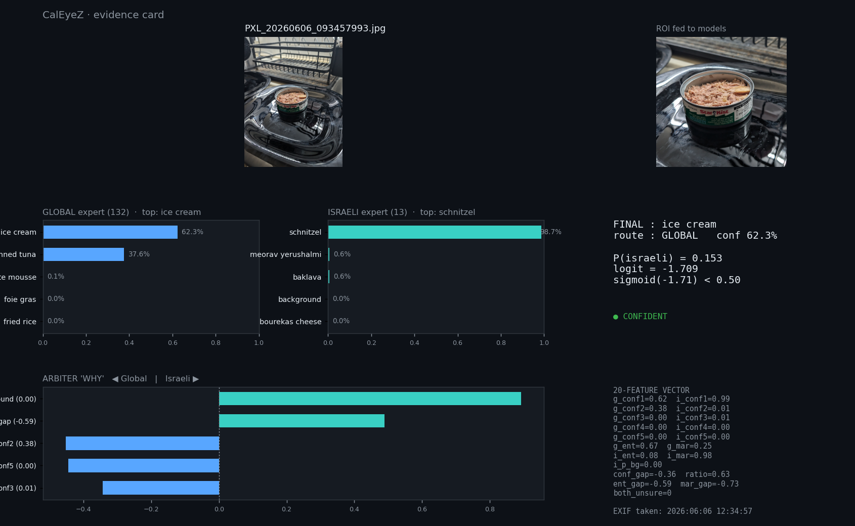
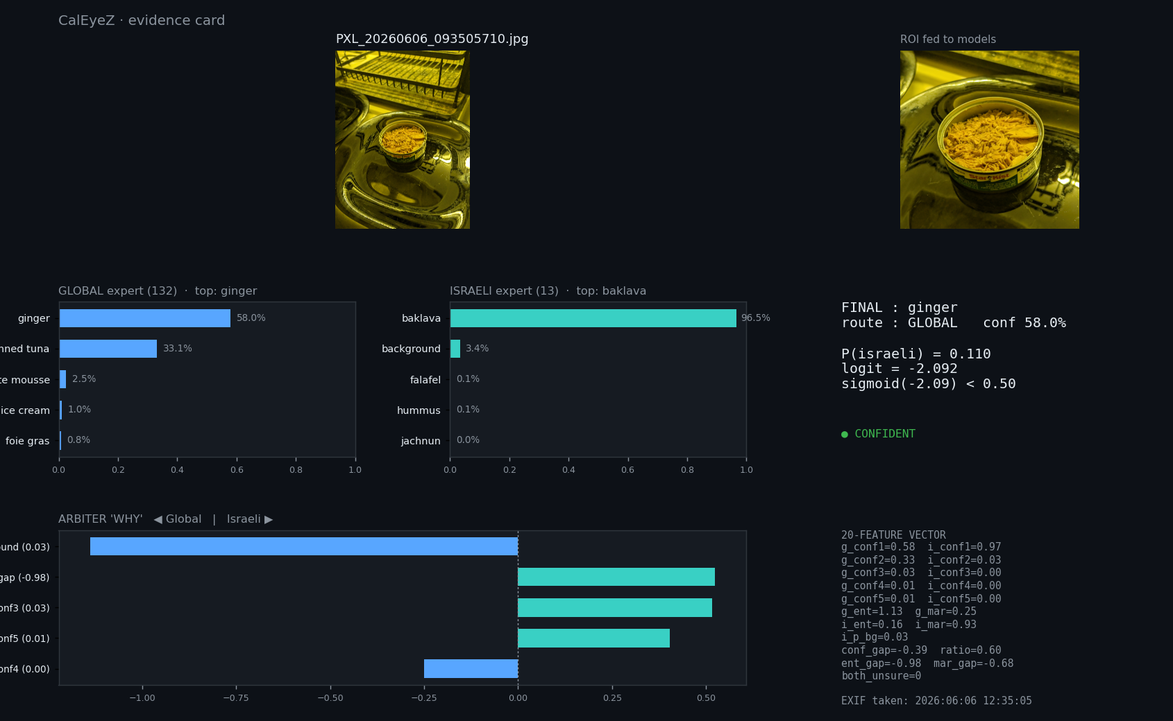
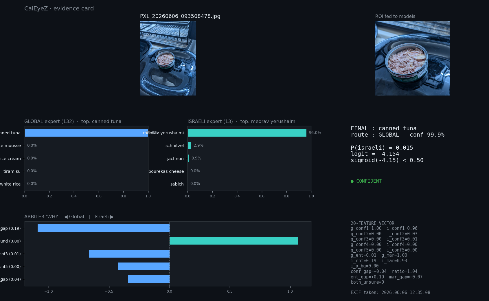
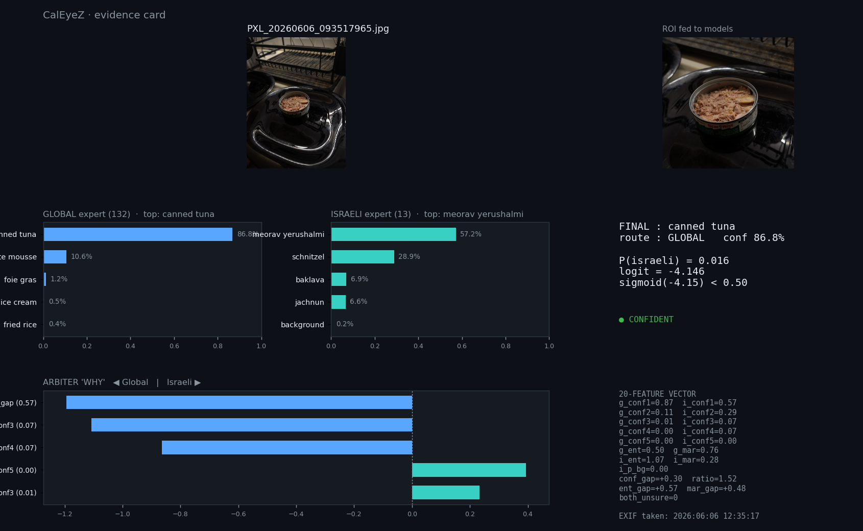
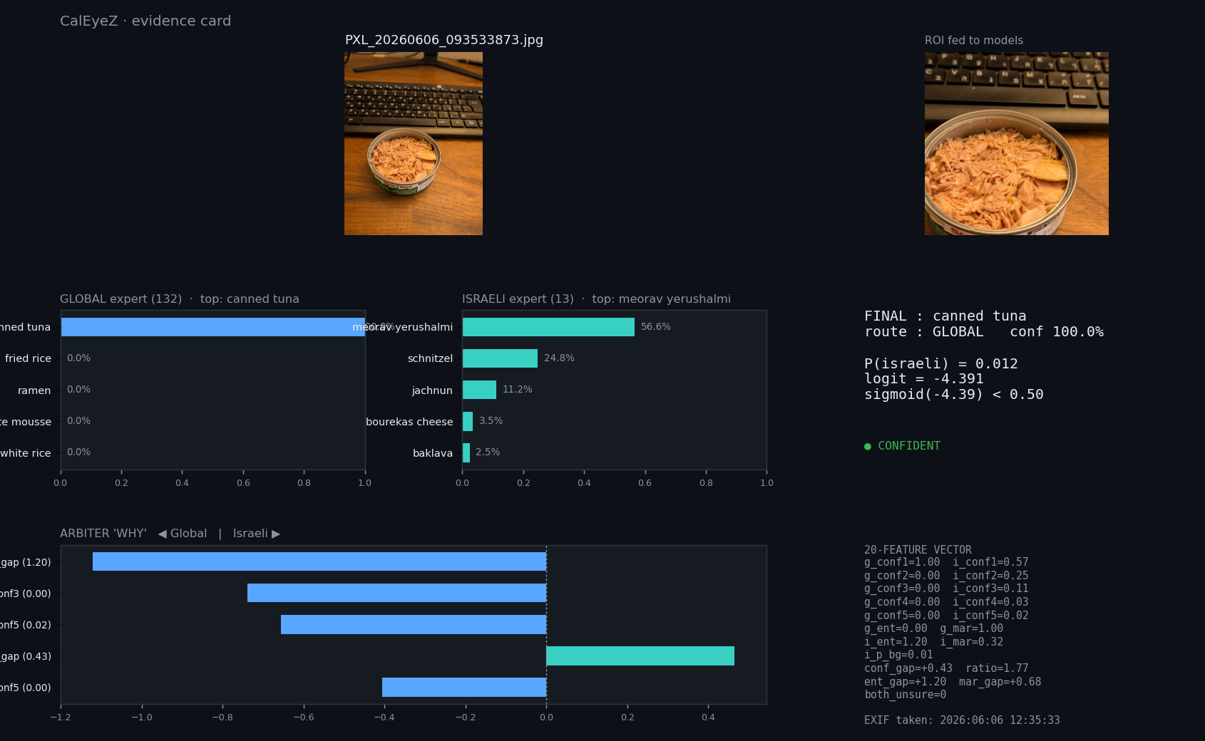
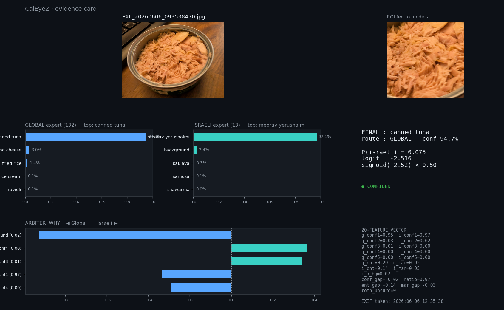
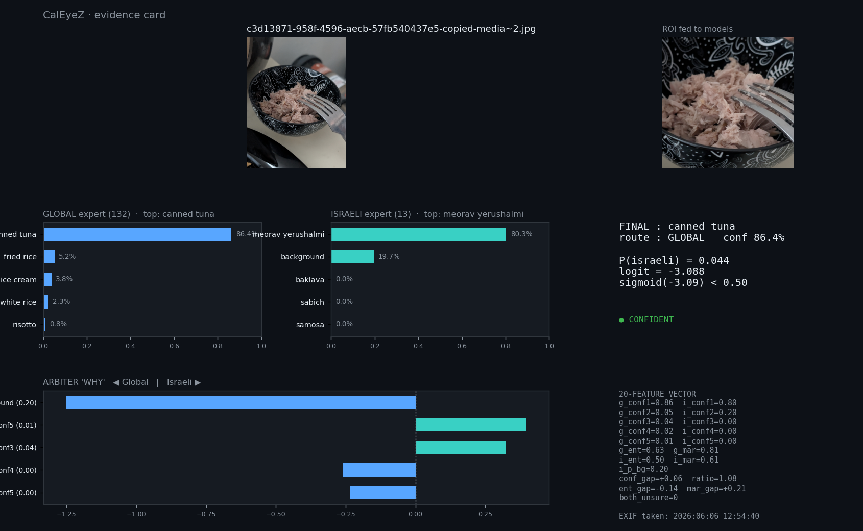
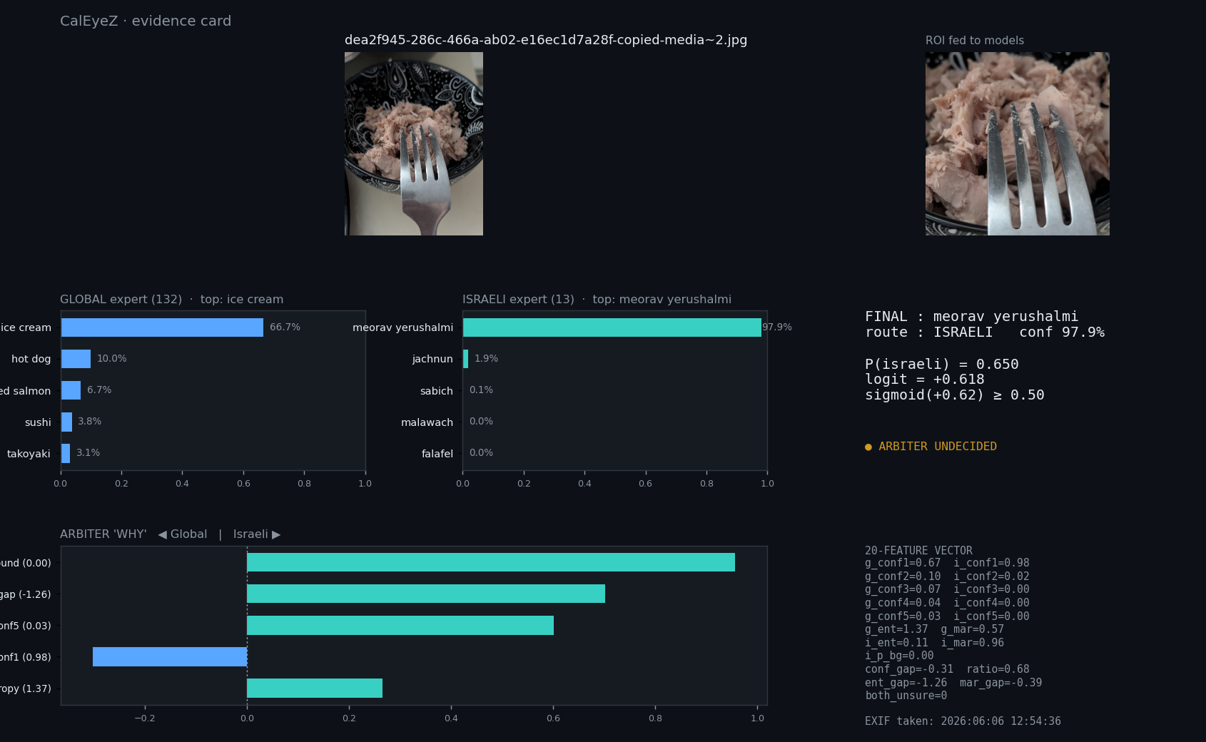
pizza
4/6 = 67%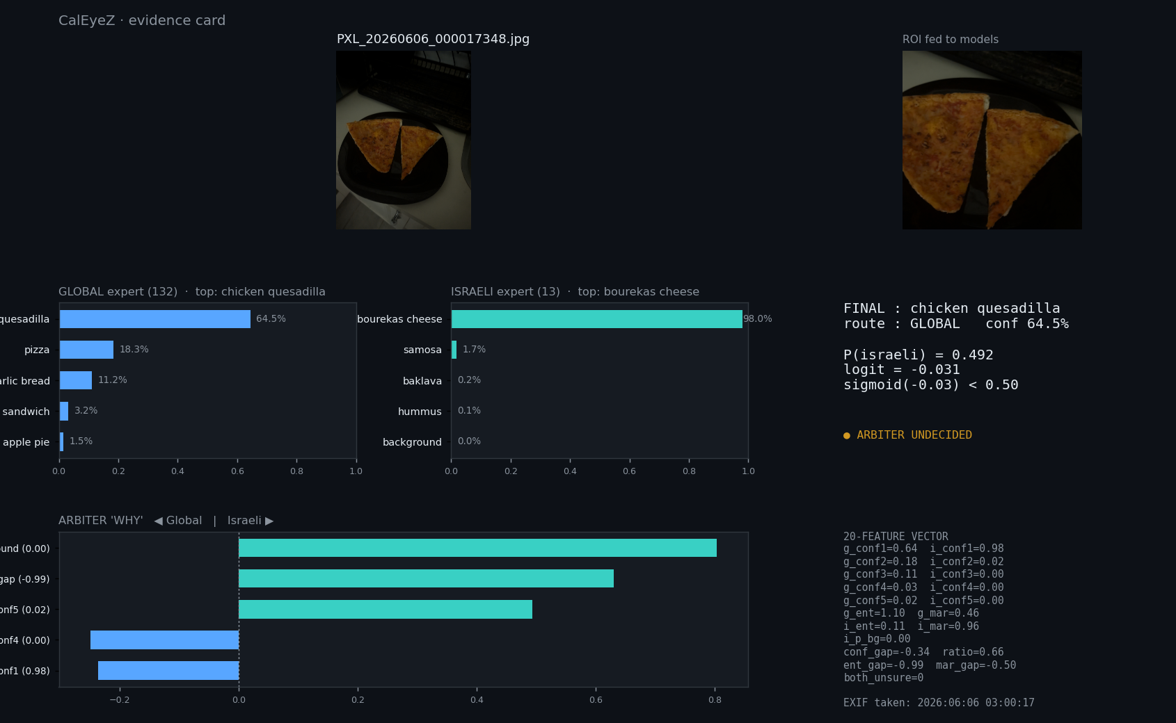
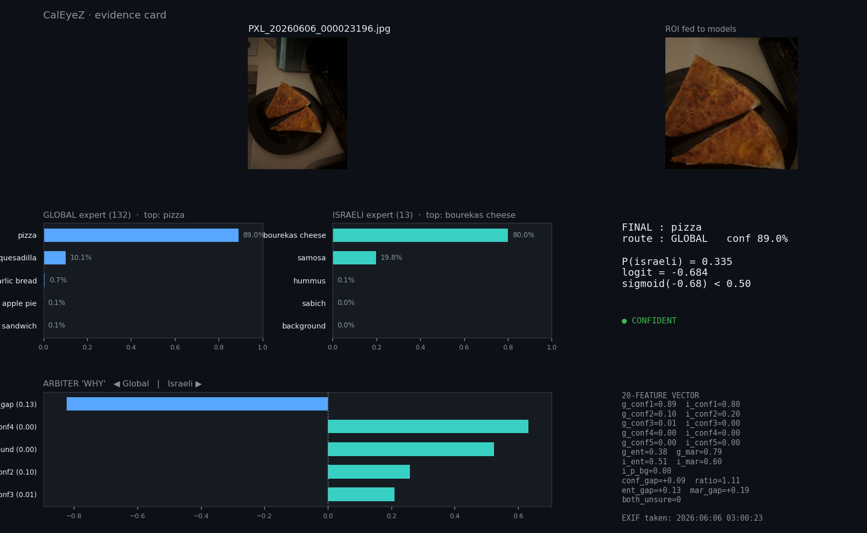
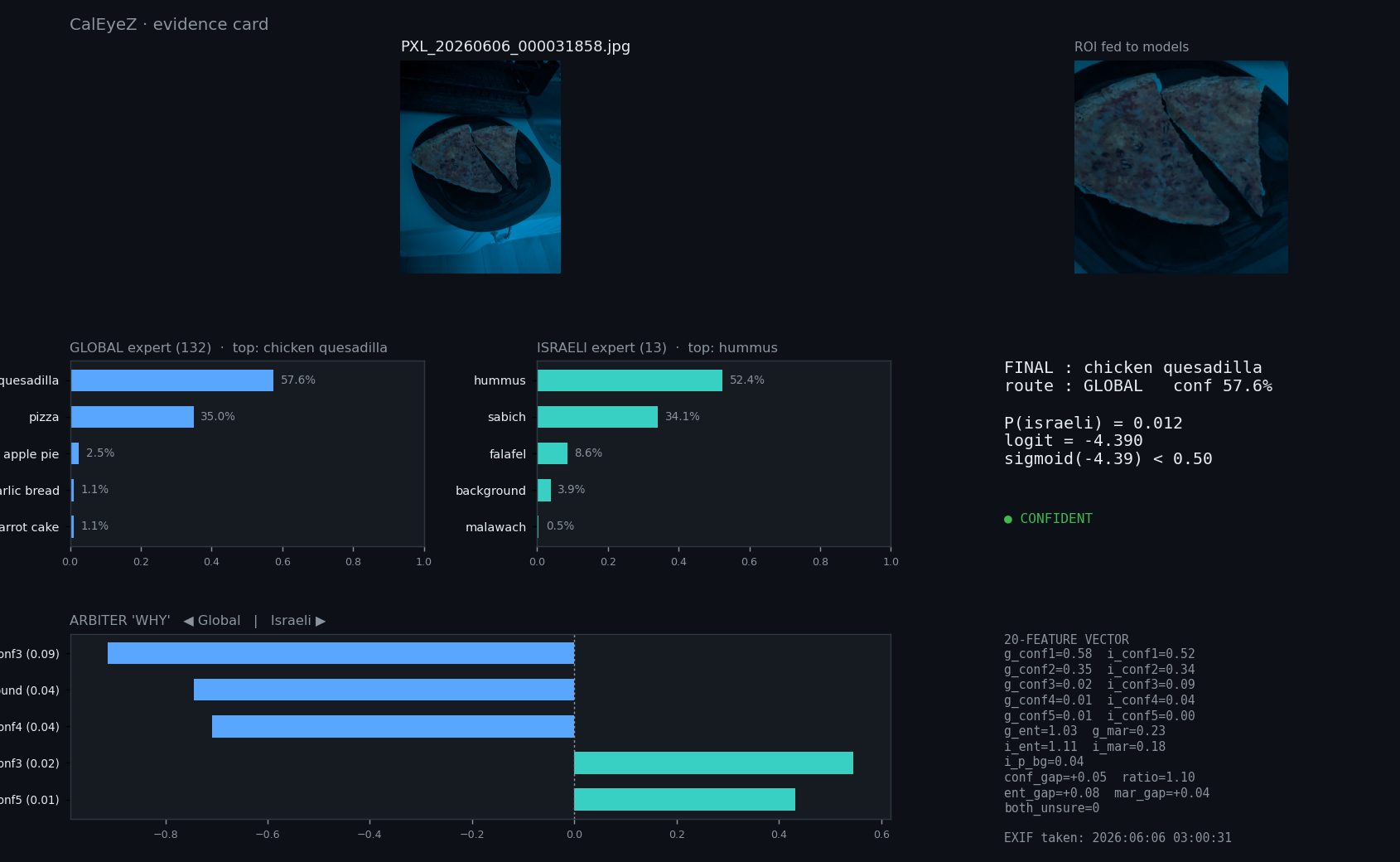
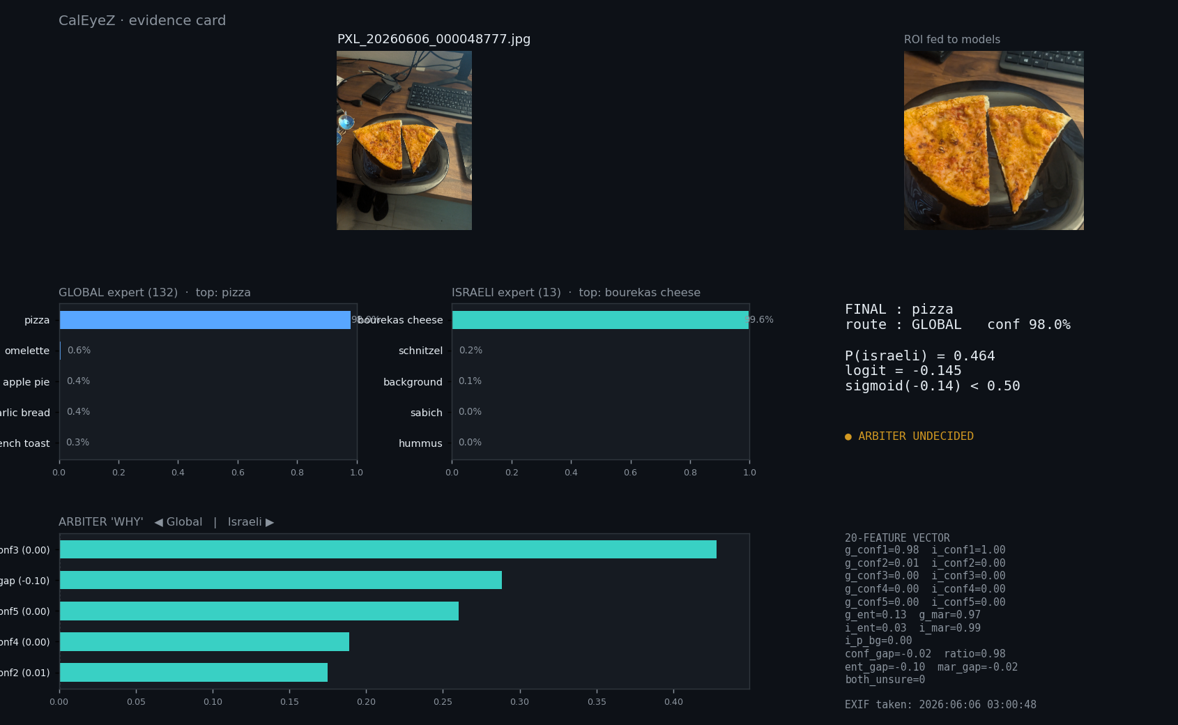
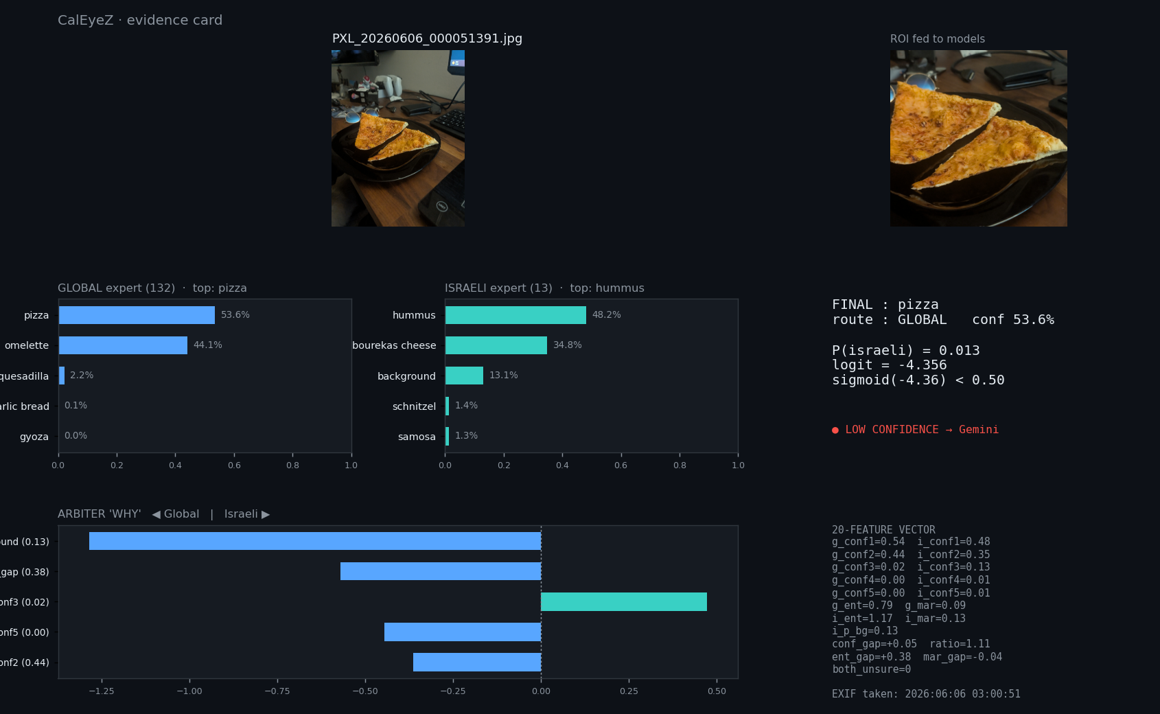
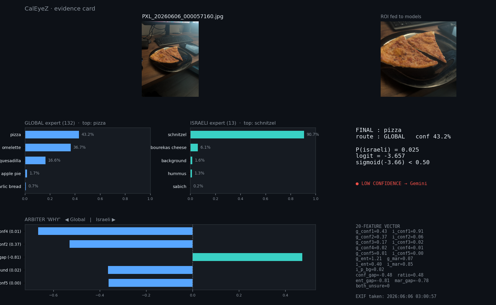
Failure modes and how I would fix them
Induced capture degradation (pizza → quesadilla)
Two pizza shots I deliberately darkened and colour-shifted collapsed to chicken_quesadilla. White-balance shift moves the colour statistics the CNN leans on.Fix: Stronger colour/temperature augmentation in training, a quick auto white-balance check at capture, and best-of-N frames in the live app.Far / top-down framing (tuna → ice cream, ginger)
A distant, top-down open can fills little of the ROI and its round rim reads as a bowl or scoop.Fix: On-screen capture guidance (fill the box, ~45° not top-down) and a multi-scale or detection-based crop so the food dominates the ROI.Within-domain Israeli look-alike (bourekas → malawach)
The Israeli expert split two genuinely similar golden fried pastries.Fix: Hard-negative mining between visually-close Israeli classes and a few more examples per dish; a fine-grained gap, not a routing one.Old low-res / re-shared images (ice cream → donuts, routing miss)
A 2015 low-resolution photo and a re-shared media file lost quality and metadata; rounded scoops read as ringed donuts and one tuna shot misrouted.Fix: Prefer recent full-resolution originals; these old/forwarded inputs are out of the deployment distribution and are kept only for honesty.CalEyeZ vs the Market - a calorie face-off
We put CalEyeZ head-to-head against the three tools people actually use, on the
same physical meals: MyFitnessPal (manual database logging), Cal.ai and
FoodVisor (AI photo estimators). Ground truth is the product label wherever one exists.
Every number below is a real trial recorded in
scripts/eval/calorie_comparison.xlsx. This is an honest pilot (small n), and
we say exactly where each number comes from.
Mean absolute calorie error over the 8 meals all three tools were tested on. CalEyeZ is the most accurate - despite MyFitnessPal being handed the true weight and a hand-picked database entry, and Cal.ai being a giant cloud model.
The decisive test: does the calorie number follow the actual portion?
The whole game is portion. The photo apps emit a typical serving; MyFitnessPal offers preset units ("1 slice", "1 can"). Both are right only when your food happens to match their assumption. CalEyeZ measures the grams on a scale, so it tracks the real portion every time. We proved it with one food, two portions:
The killer test: photograph the same food many times
Accuracy asks “how close to the truth?” - but there is a more basic question a measuring tool must pass first: repeatability. Give it the identical input twice, do you get the same answer? We took one plate of StarKist tuna and photographed it again and again, changing only the camera angle and layout - the food, and its weight, never moved.
Seven photos of one tuna plate (~31 g, truth ≈31 kcal at 104 kcal/100 g). Cal.ai’s answer swings 8× from angle alone; CalEyeZ stays on the truth line because it reads the weight off the scale, not the pixels.
Per-meal results - how close is each app to the truth?
The clearest view: for every meal, the reported calories of each app plotted right next to the grey ground-truth bar. The closer a coloured bar is to grey, the better. Below it, the same data as an absolute-error chart so small and large meals are comparable on one scale.
Reported total calories vs ground truth (grey), per meal. Ground truth is the product label where one exists. Note Cal.ai’s malawach (938 vs 393) and both-pizzas-425 overshoots, and MyFitnessPal’s tuna (309 vs 168) - each is a portion/serving guess, not a measurement.
The same eight meals as absolute % error from truth - lower is better.
The full log - every meal, every app, side by side
Each cell shows reported kcal with the % error from truth underneath. Green ✓ = the app closest to truth for that meal. “-” = the app was not tested on that meal (Cal.ai on 8, FoodVisor paywalled after one photo).
| Meal | Ground truth | Truth source | CalEyeZ | MyFitnessPal | Cal.ai |
|---|---|---|---|---|---|
| grapes | 621 | reference DB | 6342% | 6210% | - |
| bell pepper | 70 | reference DB | 5225% | 3254% | 3156% |
| cucumber | 26 | reference DB | 1831% | 1254% | 249% |
| canned tuna - full can (162 g) | 168 | product label | 1828% | 30983% | 12029% |
| french fries | 73 | recipe truth (home fries) | 172135% | 165126% | 11152% |
| hummus | 613 | product label | 37539% | 53213% | 7089% |
| Domino’s pizza | 236 | Domino’s IL data | 33542% | 18024% | 42580% |
| Pizza Hut slice | 274 | Pizza Hut data | 2615% | 18034% | 42555% |
| malawach | 393 | product label | 4258% | 3911% | 938139% |
| canned tuna - 14 g ball (portion test) | 15 | product label | 153% | - | 45209% |
| Mean absolute error (8 meals all three apps share) | 37% | 49% | 64% | ||
Per-row winners are split (CalEyeZ and MyFitnessPal each win four rows, Cal.ai two), but CalEyeZ has the lowest mean error because it never posts a catastrophic miss except french fries - and that one is a database-entry problem (generic deep-fried vs home fries), not a weight one. MyFitnessPal’s and Cal.ai’s wins come from a mature food database, which is fixable on our side; neither ever wins on measurement.
Recognition is not the same as nutrition
The axis nobody else wins: on-device, offline, instant
Cal.ai and FoodVisor stop working in airplane mode - empirical proof their inference is server-side; their 5-140 s latency is the network round-trip. CalEyeZ keeps identifying food with the network disabled, because the models run on the device itself (see Web App).
scripts/eval/calorie_comparison.xlsx · ground truth = product label where one exists.Why CalEyeZ Is Electronic Engineering, Not Just Software
A common first reaction is "this is a software project with a camera." It is not. CalEyeZ is a closed loop from the physical world, through silicon, back to a physical-world decision. Take away any one layer and a real subsystem disappears. Here is that argument laid out.
The pipeline, read as electronic-engineering stages
| Stage | What physically happens | The discipline behind it |
|---|---|---|
| Sense | A camera and a strain-gauge load cell turn light and force into electrical signals. | Sensors & Actuators · Analog Electronics |
| Condition | Median filter on the 1-D weight stream; white balance + CLAHE on the 2-D image. | Signal & Image Processing |
| Compute on silicon | Two CNNs run as tiled matrix-multiplies and convolutions, in parallel, in FP16, on a CUDA GPU. | GPU Accelerator · Computer Architecture |
| Decide | An XGBoost arbiter routes between the two experts; a confidence gate escalates when unsure. | Practical ML · Applications in AI |
| Drive it in code | OOP classes, ring buffers and bounds-checks orchestrate the camera loop and the BLE device loop. | Python for E&E · Software / C |
Each course → its project → the CalEyeZ code it produced
This is the hard proof. For every course: the project I built in it, and the actual code in our final project that the course put there. Not a name and a checkmark, the real lines.
Python Programming for E&E Engineers · תכנות פיתון למהנדסי חשמל
What it put into CalEyeZ
The CalEyeZ code
# scripts/demo/caleyez_demo.py - the module library + a hardware device
import cv2, numpy as np, pandas as pd
from PIL import Image, ImageTk
from bleak import BleakScanner, BleakClient   # BLE hardware, in pure Python
...
self.cap = cv2.VideoCapture(0)   # a physical camera
self._tick_camera()                # live frame loop
self._tick_weight()                # live weight loop from the BLE scale
Immediate impact
The course's thesis, "intelligent operation of any hardware component", is literally the live demo: a camera loop and a BLE device loop running together in one Python program.Software - Programming in C · מבוא למדעי המחשב (C)
What it put into CalEyeZ
The CalEyeZ code
# scripts/demo/caleyez_demo.py - a class that inherits and overrides, and the app object
class AutocompleteEntry(tk.Entry):                 # inherits a base class
    def __init__(self, parent, textvar, options, **kw):
        super().__init__(parent, textvariable=textvar, **kw)
class CalEyeZDemo:
    def __init__(self, root):
        self.frames = deque(maxlen=6)   # fixed-size buffer = the array/struct discipline from C
Immediate impact
Pointers, dynamic memory and bounds-checking from C are the exact mental model for reasoning about GPU memory and array indexing later. This course is the floor the GPU work stands on.GPU Parallel Hardware Accelerator · חומרה מאיצה (GPU / CUDA)
★ The beating heart. The two vision models exist only because a GPU runs convolutions and matrix-multiplies in parallel, the precise subject of this course.
What it put into CalEyeZ
The CalEyeZ code
# scripts/training/train_general_model.py - CUDA GPU + FP16
results = model.train(
    device = 0,          # the CUDA GPU
    amp    = True,       # mixed precision = the FP16 path from the floating-point lecture
)
# scripts/demo/caleyez_demo.py - a GPU forward pass (the "Deep Learning on GPU" lecture)
g = model_g.embed(roi, imgsz=GLOBAL_IMGSZ)[0]  # 512-D penultimate features, on the GPU
My course project → why it IS this engine
CUDA Attention Mechanism - Transformer attention written from scratch in CUDA
I hand-wrote and optimized the same primitives the YOLO models run millions of times per image:
| Implementation | Time (N=512) | Speed-up |
|---|---|---|
| CPU reference | 36.465 ms | 1× |
| Basic GPU (4 kernels) | 0.612 ms | ≈60× |
| Optimized GPU (tiled + fused) | 0.170 ms | ≈214× vs CPU |
// attention.cu - the optimized fused QKᵀ kernel
#define TILE 32                          // = NVIDIA warp size → coalesced access
__global__ void qkt_fused_opt(const float* Q, const float* K, float* S, float scale){
  __shared__ float Qs[TILE][TILE], Ks[TILE][TILE];
  Ks[ty][tx] = (col < N && kK < D) ? K[col * D + kK] : 0.0f;  // virtual transpose + guard
  for (int k = 0; k < TILE; ++k) acc += Qs[ty][k] * Ks[k][tx];
  if (row < N && col < N) S[row * N + col] = acc * scale;   // KERNEL FUSION
}
Impact on CalEyeZ: a YOLO layer is this kernel at scale. Having built and profiled the tiled/fused matmul myself, the amp=True training run and GPU forward passes are not a black box, they are the production version of the kernel I wrote.
Foundation: Computer Architecture (3602801)
The GPU work is legible only because of the Von-Neumann model and the register-vs-memory latency hierarchy (registers ≈ 1 cyc, shared ≈ 5, global ≈ 500) that is the whole reason for tiling into shared memory.| CPU revision | Cycles | Technique |
|---|---|---|
| Basic single-cycle MIPS | 53 | standard fetch/decode/execute loop |
| Extended ISA | 6 | custom ALU op (func 101011) = n(n+1)/2 − m(m−1)/2 in hardware |
| Minimal 2-cycle | 2 | stripped datapath, dedicated accumulator |
| Pure combinational | 0 | clockless logic, result instant |
Impact: designing a datapath and extending an instruction set is the same instinct behind choosing FP16 tensor paths and fused CUDA kernels above. A GPU is this machine, massively parallelised.
scripts/training/train_general_model.py, train_israeli_food_v2.py, scripts/demo/caleyez_demo.py.Practical Machine Learning · למידת מכונה יישומית
What it put into CalEyeZ
The CalEyeZ code
# scripts/training/train_israeli_food_v2.py - supervised deep learning + calibration
model = YOLO("yolo11l-cls.pt")
results = model.train(
    data=DATASET_DIR, task="classify",
    epochs=120, patience=25,        # early-stop on val top-1 = no overfitting
    label_smoothing=0.1,           # calibrated, trustworthy probabilities
)
My course project → the methodology it taught
Predictive Data-Science Pipeline for USA Housing Prices
| Stage | Best model | R² |
|---|---|---|
| Raw features | Linear regression | 0.33 |
| After feature engineering | Linear / Ridge | 0.77 |
| Non-linear | Random Forest | 0.98 |
Impact on CalEyeZ: identical discipline, leakage-free splits and metric-driven decisions, applied to images instead of tables. It also taught me when feature engineering beats a fancier model, which directly shaped the hand-built 20-feature arbiter vector.
scripts/training/train_israeli_food_v2.py, train_general_model.py · Results: runs/*/confusion_matrix.png.Contents & Applications in Artificial Intelligence · יישומים בבינה מלאכותית
What it put into CalEyeZ
scale_pos_weight for imbalance, ROC-AUC, and a baseline-vs-oracle trade-off study.The CalEyeZ code
# scripts/arbiter/train_arbiter_xgb.py - a boosted decision-tree ensemble + honest eval
clf = xgb.XGBClassifier(n_estimators=400, max_depth=5, learning_rate=0.05,
    scale_pos_weight=spw, eval_metric="auc")        # class imbalance handling
auc        = roc_auc_score(yte, proba)            # characterise the model
routed_acc = routed_correct.mean()                # vs an always-global baseline…
oracle_acc = (g_corr | i_corr).mean()             # …and the perfect-router ceiling
My course project → the arbiter's algorithm family
Decision-tree & ensemble modelling (from the Housing-Price pipeline)
Impact on CalEyeZ: reading decision-tree splits is exactly how the arbiter routes, a learned hierarchy of threshold splits on the 20 features. The XGBoost choice is a deliberate one I understand from the inside, not a black box.
scripts/arbiter/train_arbiter_xgb.py, generate_arbiter_dataset.py.Sensors and Actuators · חיישנים ומפעלים
What it put into CalEyeZ
The CalEyeZ code
# scripts/ble/scale_reader.py - raw transducer bytes → grams, with a stability spec
low_byte  = hex_data[4]
high_byte = hex_data[5] | hex_data[3]          # full high byte = number of 256s (no mask)
weight = sorted(raw_buffer)[len(raw_buffer)//2]      # MEDIAN filter = noise vs responsiveness
delta  = max(stability_buffer) - min(stability_buffer)
software_stable = delta <= STABILITY_THRESHOLD        # ≤2 g over 10 samples ⇒ STABLE
My course project → the same trade-offs in hardware
Portable Metal-Detector Circuit
Impact on CalEyeZ: this is where sensitivity vs linearity and accuracy vs sampling rate became physical realities of a transducer, the exact trade-offs the BLE scale's median filter + stability gate implement above.
Analog foundation: Analog Electronics & VLSI
A strain-gauge load cell outputs microvolts; recovering it needs the differential amplification and offset behaviour I designed in the op-amp project, and the scale + BLE radio run on the kind of on-chip oscillator I characterised. These are the analog physics that make "read grams over Bluetooth" possible.
scripts/ble/scale_reader.py; same protocol in scripts/demo/caleyez_demo.py.Signal & Image Processing · עיבוד אות ותמונה
What it put into CalEyeZ
The CalEyeZ code
# scripts/demo/caleyez_demo.py - 2-D image filtering before recognition
def center_roi(bgr):
    h, w = bgr.shape[:2]
    s = int(min(h, w) * ROI_FRAC)        # deterministic 2-D crop
    y0, x0 = (h - s)//2, (w - s)//2
    return bgr[y0:y0+s, x0:x0+s].copy()
# scripts/ble/scale_reader.py - the SAME course's 1-D filtering, on the sensor signal
weight = sorted(raw_buffer)[len(raw_buffer)//2]   # median = a non-linear 1-D digital filter
Immediate impact
The same filtering instinct cleans the camera image (2-D) and the scale's weight stream (1-D). The convolution the GPU course accelerates is the very operation this course defines.scripts/demo/caleyez_demo.py (image front-end), scripts/ble/scale_reader.py (1-D filter).Recap: course → subsystem → proof
| # | Course | Subsystem it became | Proof in the repo |
|---|---|---|---|
| 1 | Python for E&E | The whole hardware-driving program | caleyez_demo.py |
| 2 | Software / C (OOP) | Classes, buffers, algorithms, bounds-checks | caleyez_demo.py |
| 3 | GPU Accelerator (CUDA) | The GPU that runs the models (FP16, convolutions) | train_general_model.py |
| 4 | Practical ML | Two supervised deep-learning classifiers | train_israeli_food_v2.py |
| 5 | Applications in AI | The XGBoost decision-tree arbiter / router | arbiter/train_arbiter_xgb.py |
| 6 | Sensors & Actuators | The BLE load-cell scale + stability spec | ble/scale_reader.py |
| 7 | Signal & Image Processing | 1-D weight filter + 2-D image normalisation | caleyez_demo.py · scale_reader.py |
| + | Computer Architecture | Von-Neumann/FDE model behind the GPU + a MIPS CPU in Verilog | folded into ③ · MIPS project |
Per-Class Performance
The 86.16% system figure is an average. This view breaks it down to every one of the 145 classes: its recall on the held-out test set, the food it is most confused with, and why. This is where the real limitations live.
Reading it: recall = the share of that class's test images identified correctly, so 75% recall means 25% were missed. But recall on a tiny test set is noisy: a class with only 8 images moves 12.5% per single miss, so those numbers carry a wide 95% confidence interval and should not be ranked literally. Use reliable only (n ≥ 50) to see the weaknesses that are statistically real.
| Class | Recall | n (test) | Most confused with | Why |
|---|
The Voice-Fingerprint Analogy
CalEyeZ is a convolutional neural network, but you can understand exactly what it does without any deep-learning vocabulary - just signals and filters. Imagine building a system that recognises who is speaking. That system and CalEyeZ are the same machine; only the input changes from a voiceprint to a food photo.
The story, step by step
Collect many voices, all speaking the same language
We record many people speaking, say, English. Each raw recording is just a pressure wave - far too much data to compare directly. We need to boil every voice down to a few numbers that capture what makes it that voice.
Pass each voice through a bank of filters
Classic signal processing gives us band-pass filters (IIR, Butterworth, …). Each one isolates one aspect of the sound: the pitch (fundamental frequency f0), the timbre, the speaking cadence, the loudness, the vowel formants. The difference here is that these filters are not hand-designed with fixed coefficients - they start random and are learned from the data. In a CNN these "filters" are the convolution kernels, and the stack of them is called the backbone.
Training tunes the filters - but only the final answer is graded
This is the one place the intuition needs care. We do not tell the network the "true pitch" or "true timbre" of each voice - there is no measured target for the intermediate features. The only thing we grade is the final guess: did it name the right speaker? We measure how wrong that guess was (the loss) and backpropagation pushes that single error backwards through every filter, nudging each one a little at every epoch. Over many epochs the filters self-organise to extract whatever features make the final answer correct. They discover "pitch and timbre matter" on their own - nobody hands them that.
The output is a vector - the voice's "DNA"
After the filter bank, each voice is reduced to a short list of numbers, v = {pitch, timbre, cadence, loudness, …}. This vector is the fingerprint of that voice. In CNN terms it is the embedding (or feature vector).
Recognition: dot-product against every learned template
To recognise a new voice, we run it through the very same filters to get its vector v. The final layer stores one learned template (a weight vector) for every speaker it knows. We take the dot product of v with each template and add a bias: z_c = w_c · v + b_c. The bigger the dot product, the more the input lines up with that speaker's template. Those raw scores z (e.g. 4.1, 2.0, 1.1, 0.3) are the logits.
Softmax turns scores into probabilities
Logits are unbounded numbers, not probabilities. Softmax exponentiates each one and normalises so they sum to 1:
The largest probability is the system's answer. That is the entire recognition pipeline.
Adding a second accent - the catastrophic-forgetting problem
Now suppose we want the same system to also recognise Israeli speakers. They use the same physics of speech, but the statistics differ - louder on average, different cadence and formants. We have three options:
| Option | What you change | Result |
|---|---|---|
| 1 · Retrain all filters | Re-tune the whole backbone on Israeli voices. | The filters drift to fit the new voices and forget the English ones - catastrophic forgetting. We measured exactly this and rejected it. |
| 2 · Fine-tune only the head | Freeze the filters; only re-weight the features (e.g. trust cadence ×10, loudness ×0.5). | Standard transfer-learning fix. Cheap, keeps old knowledge, but limited if the new domain really needs different features. |
| 3 · Two specialists + a router | Keep the English expert untouched, train a separate Israeli specialist, and add a learned router that decides per input which expert to trust. | What CalEyeZ does. No forgetting, and each expert stays sharp on its own domain. |
CalEyeZ took option 3. The Israeli specialist even carries an extra "background / not-mine" class, so when an English voice reaches it, it can say "this isn't mine" - which is the strongest signal the router uses to send the input back to the English expert.
The reverse case is just as important: feed an English food and the Israeli expert returns a high P(background) ("not mine") with low confidence, so the router sends the decision to the Global expert instead. That single "not-mine" signal is the top feature in the real arbiter and is why routing reaches ROC-AUC 0.973.
How this maps onto CalEyeZ - exactly
| Voice analogy | CalEyeZ (the real system) |
|---|---|
| Raw voice recording | Raw food photo (RGB image) |
| Band-pass filters (IIR/Butterworth) | Convolution kernels (learned filters) |
| The whole filter bank | The CNN backbone (YOLO11l-cls feature extractor) |
| Filters auto-tuned by the final error | Backpropagation of cross-entropy loss (with label smoothing ε=0.1) |
| Voice DNA vector v | The image embedding / feature vector |
| Dot product with each speaker template | Final classification layer: z_c = w_c · v + b_c |
| Raw scores z | Logits (one per food class) |
| Softmax → probabilities | Softmax → per-class confidence (132 global / 13+1 Israeli) |
| 132 English speakers | 132 international food classes (Global model) |
| Israeli speakers + "not-mine" class | Israeli specialist: 13 dishes + open-set "background" class |
| Catastrophic forgetting when retraining all filters | Exactly why we did not extend the Global model - measured and rejected |
| Router choosing which specialist to trust | XGBoost arbiter (20 features, ROC-AUC 0.973) |
The analogy is exact except for one subtlety worth stating: in pure DSP you could measure pitch directly and tune a filter against that measured value. A CNN cannot - there is no ground truth for any intermediate feature. The network is graded only on the final class, and the filters are shaped indirectly by backpropagating that final error. So "we fine-tune the filters" is true, but the teacher is the answer at the end, never the features in the middle.
Want to see the softmax math live (drag the logits and watch the probabilities, entropy and margin update)? Open the Training Lab. Want the routing decision explained per image? See the Arbiter tab.